
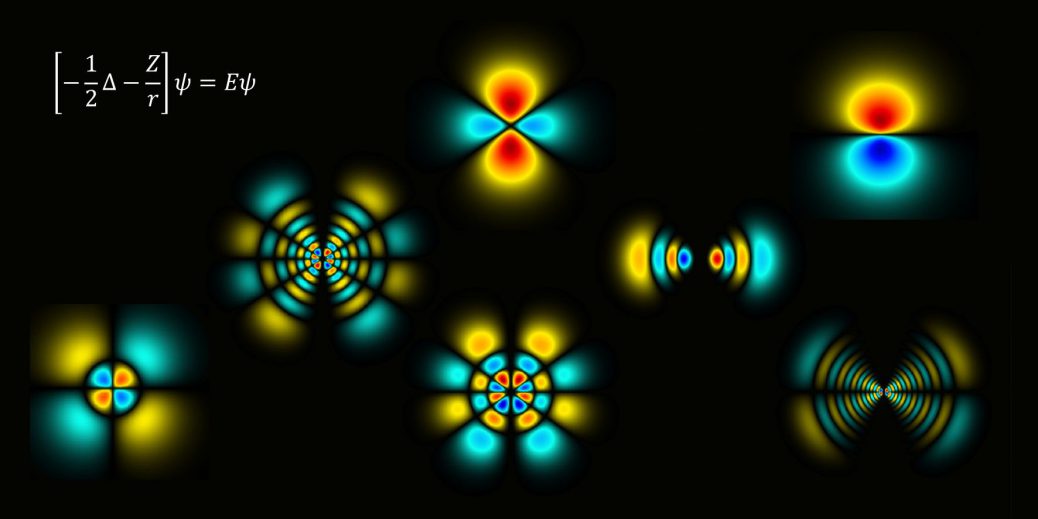
非相対論的な水素様原子の電子の波動関数を求めるfortranコードを書きます。
解く問題
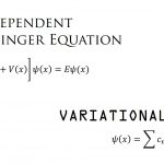
電荷\(+Ze\)の原子核の周りに存在する、電荷\(-e\)を持つ電子が満たす時間依存しないシュレーディンガー方程式は、
\(
\displaystyle \left[-\frac{1}{2}\Delta-\frac{Z}{r}\right]\psi({\bf r})=E\psi({\bf r})
\)
です。
\(
\left. \psi({\bf r})\right|_{|{\bf r}|\to \infty}\to 0
\)
の境界条件を満たす正規直交化された解は、
\(
\begin{align}
\psi({\bf r})&=R_{n,l}(r)\cdot Y_{l,m}(\theta,\varphi)\\
&=\sqrt{\left(\frac{2}{n}\right)^3\frac{(n-l-1)!}{2n[(n+l)!]}} e^{-Zr/n} \cdot \left(2\frac{Zr}{n}\right)^l\cdot L_{n-l-1}^{(2l+1)}\left(2\frac{Zr}{n}\right)\cdot Y_{l,m}(\theta,\varphi)
\end{align}
\)
と表されます。ここで、
- \(n,l,m\) 主量子数,方位量子数,磁気量子数
- \(r,\theta,\varphi\) 動径方向,z軸方向の角度,xy平面の角度
- \(L_n^{(\alpha)}(x)\) ラゲール陪多項式[1]
- \(Y_{l,m}(\theta,\varphi)\) 球面調和関数[2]
を意味します。
動径関数\(R_{n,l}(r)\)は微分方程式
\(
\displaystyle \left[-\frac{1}{2}\left(\frac{d^2}{dr^2}+\frac{2}{r}\frac{d}{dr}\right)+\frac{l(l+1)}{2r^2}-\frac{Z}{r}\right]R_{n,l}(r)=E_n R_{n,l}(r)
\)
を満たす正規直交化された関数で、固有値は
\(
\displaystyle E_n=-\frac{1}{2n^2}
\)
です。
波動関数を出力するFortranコードはこれ。
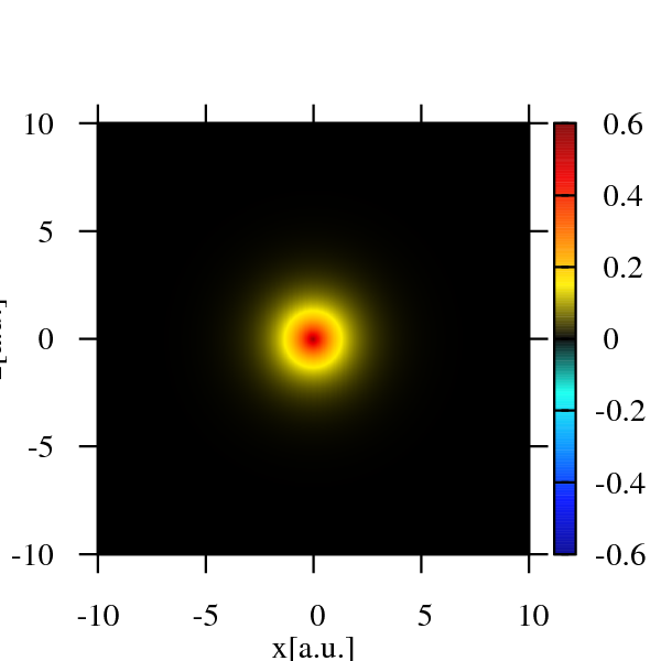
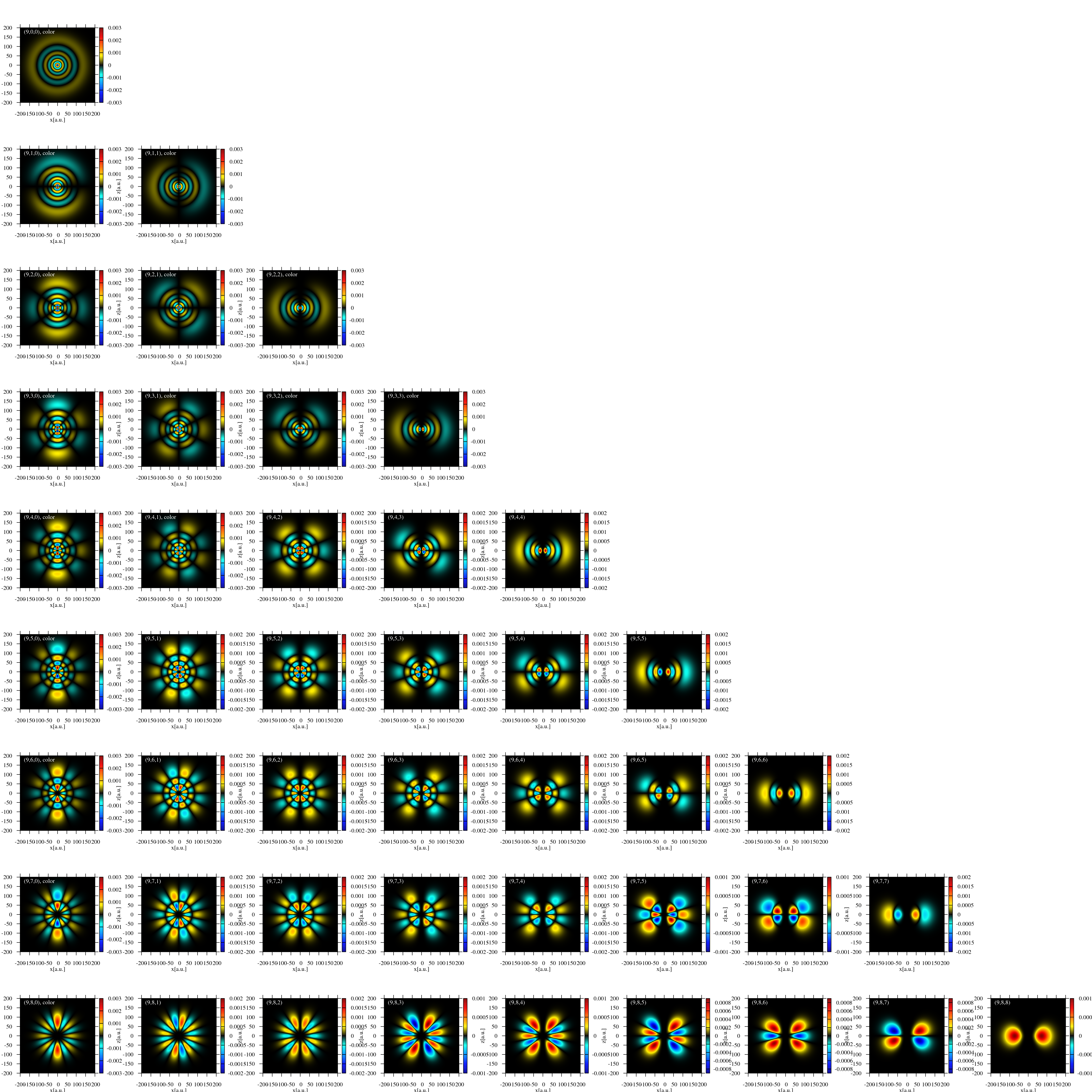
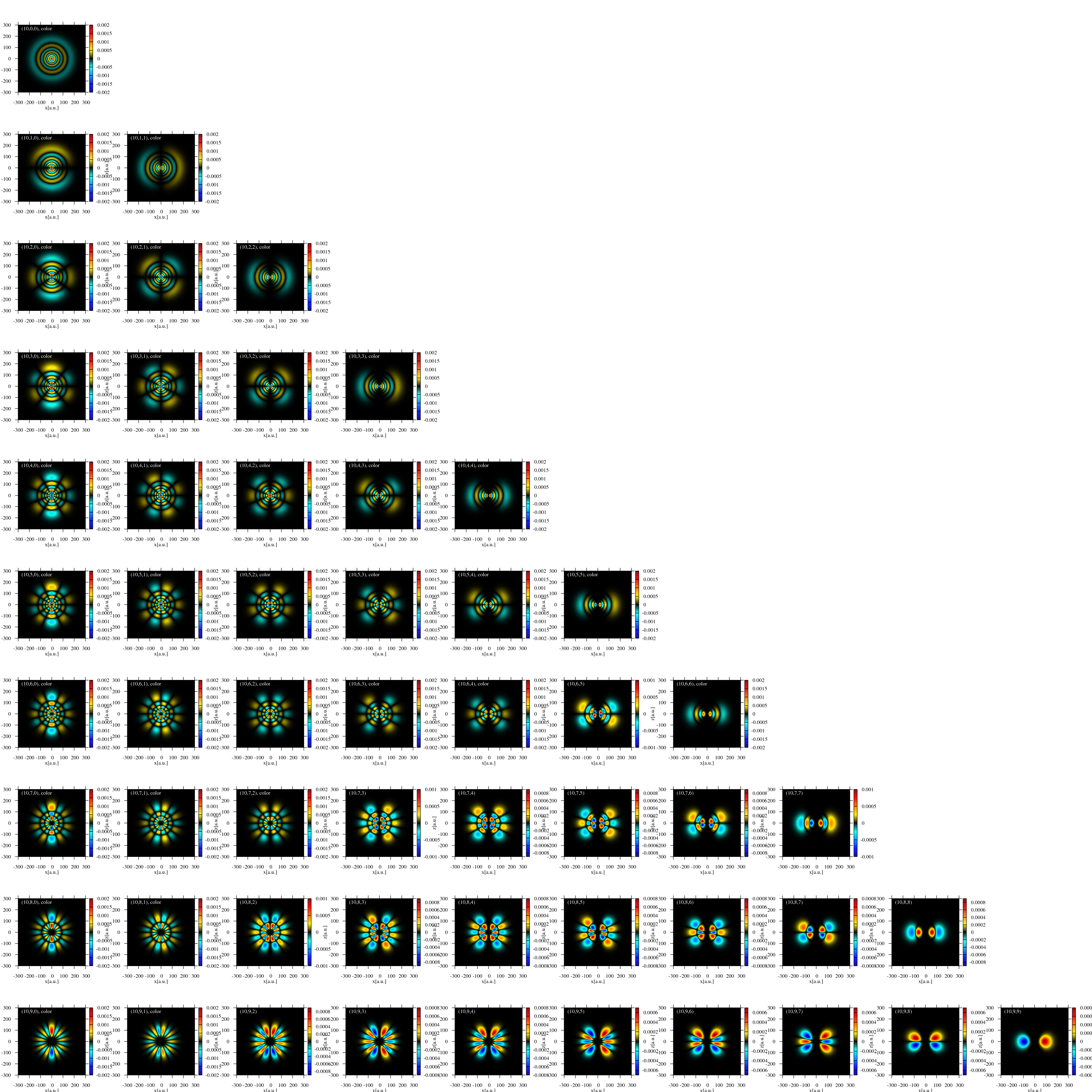
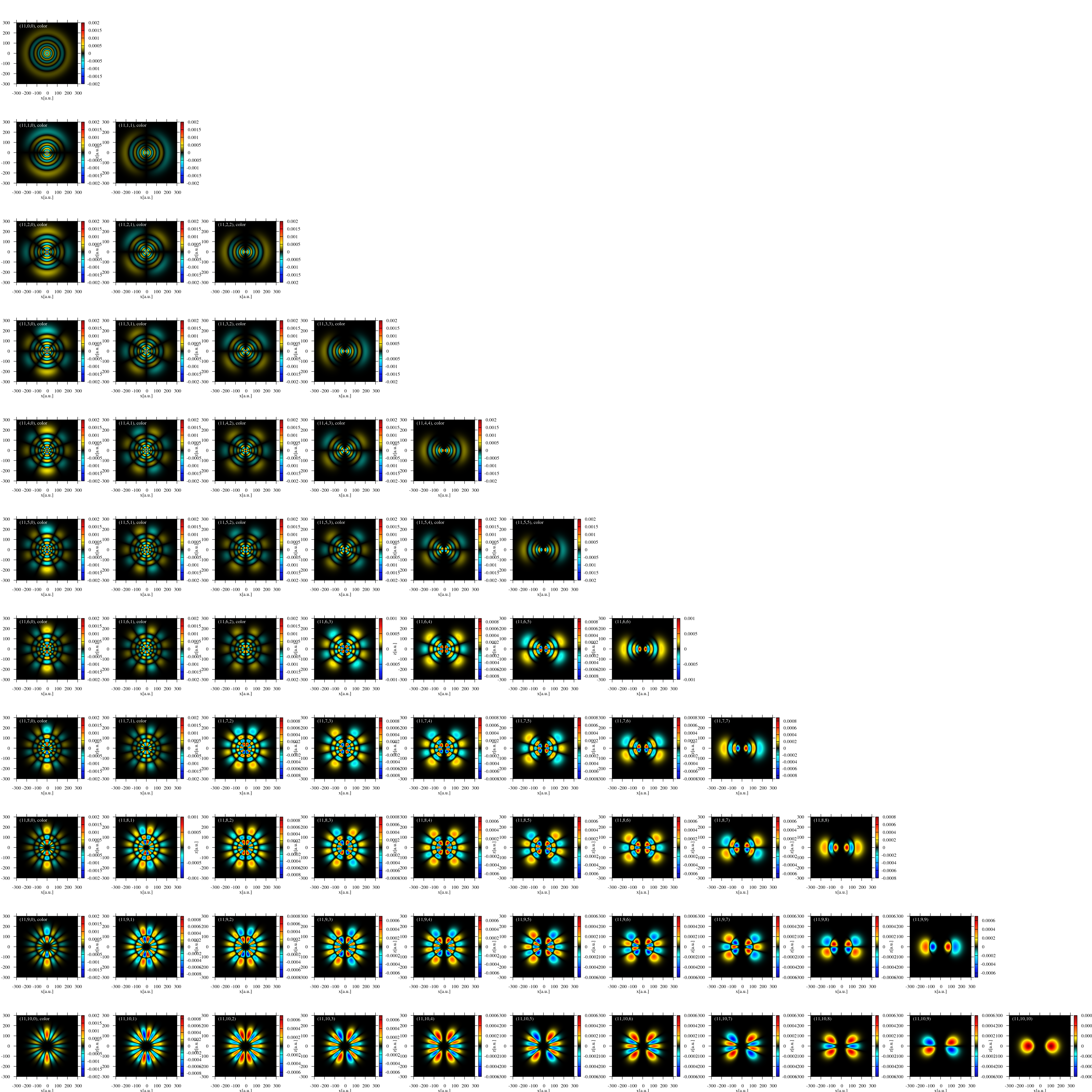
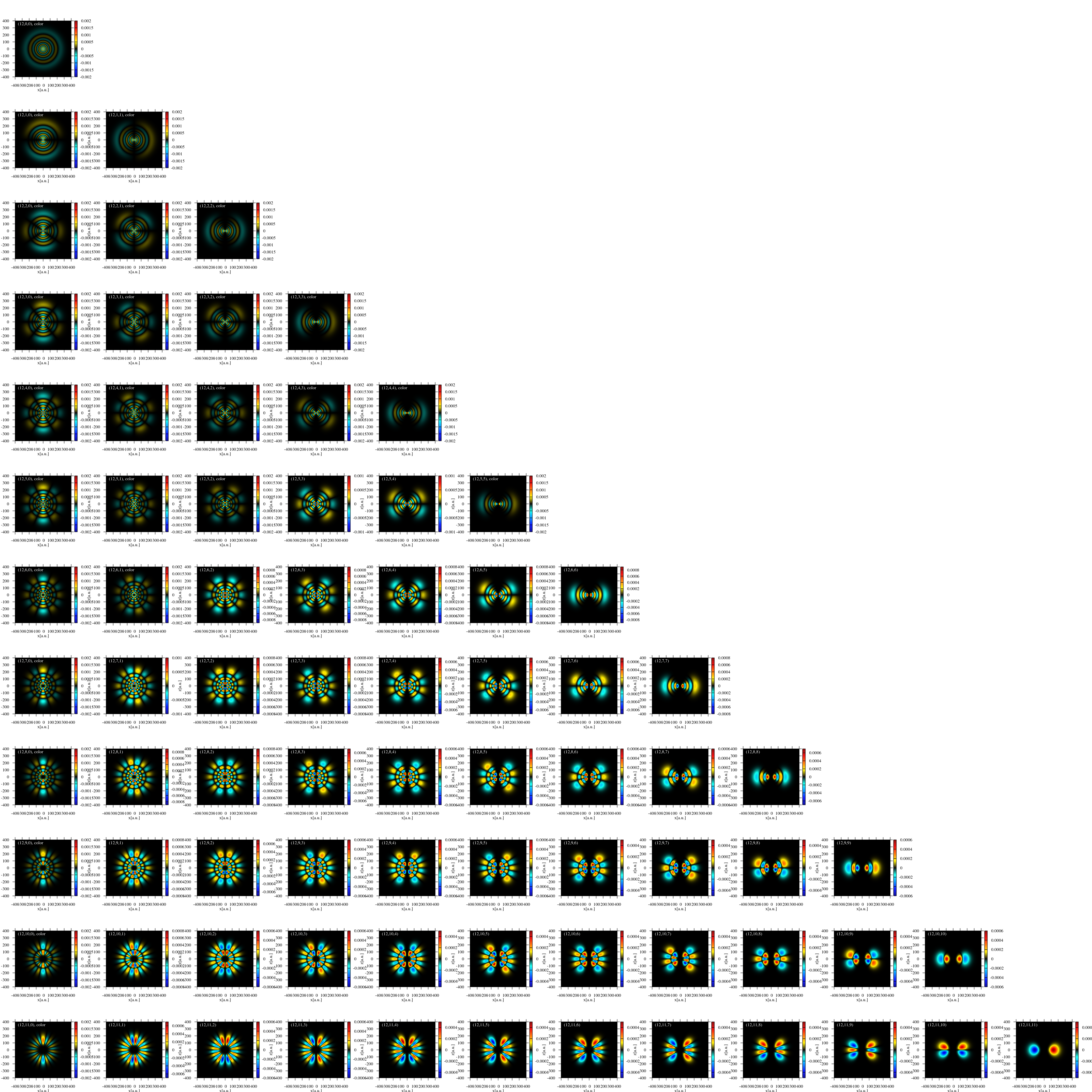
計算結果
3次元の波動関数を表示するには3つの座標と波動関数の値の計4つが必要です。
しかし、4次元空間を分かりやすく描画する方法はありません。
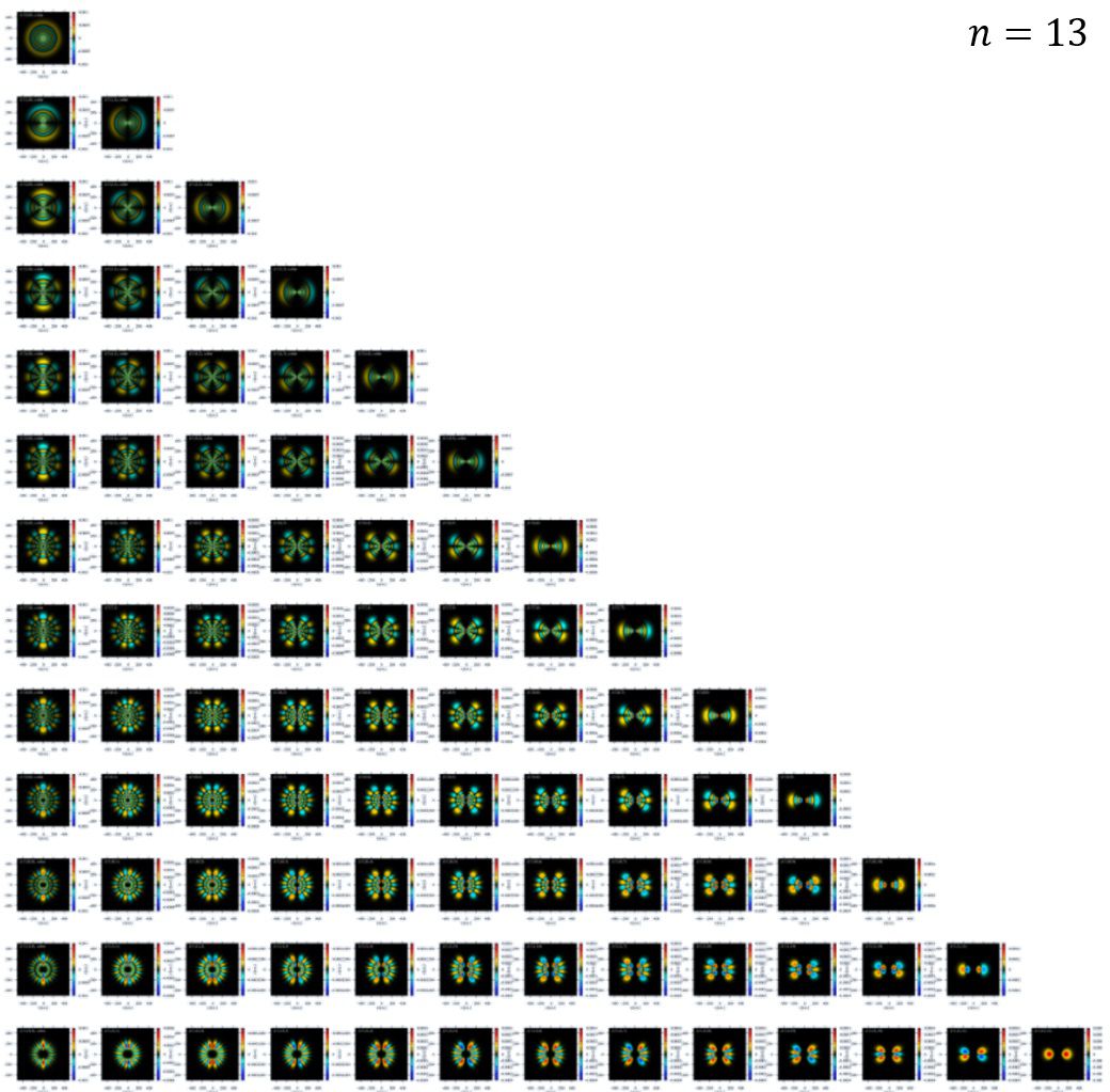
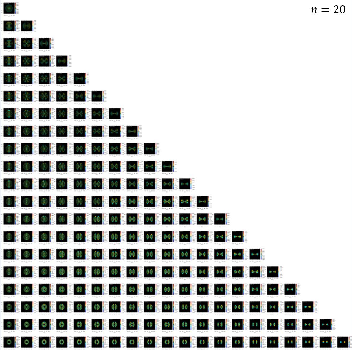
そこで、ここでは\(\mathrm{Re}{\psi(x,0,z,t)}\)のように、\(y=0\)にしてグラフを描画します。
\(z\)軸周りの構造がうまく表現できませんが、良しとします。
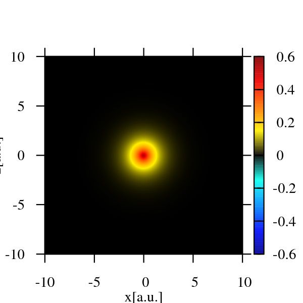
\(n=1\)
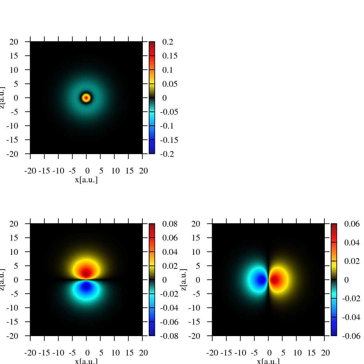
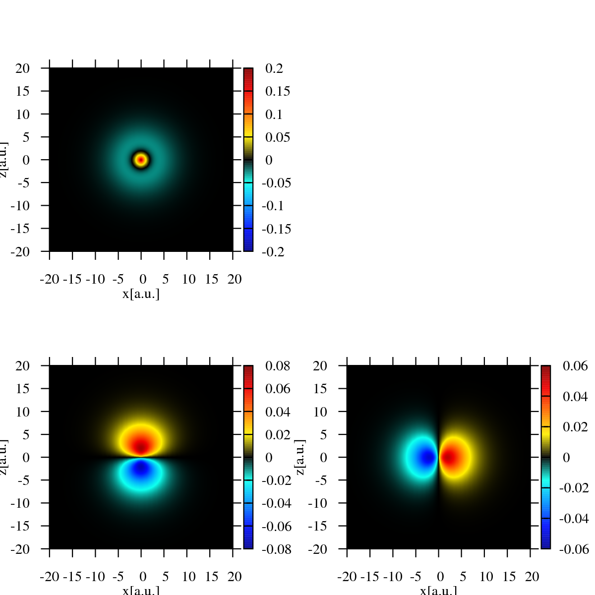
\(n=2\)
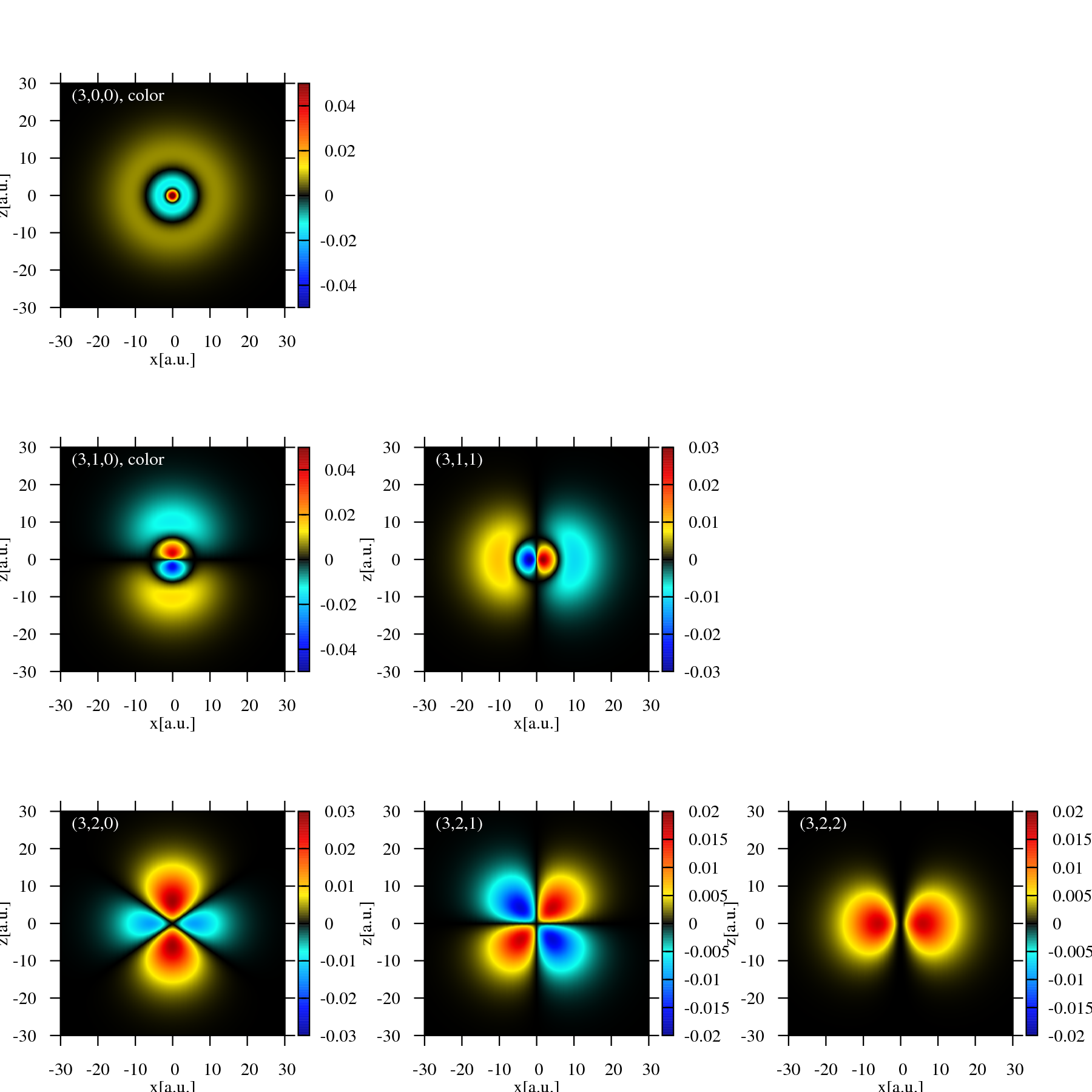
\(n=3\)
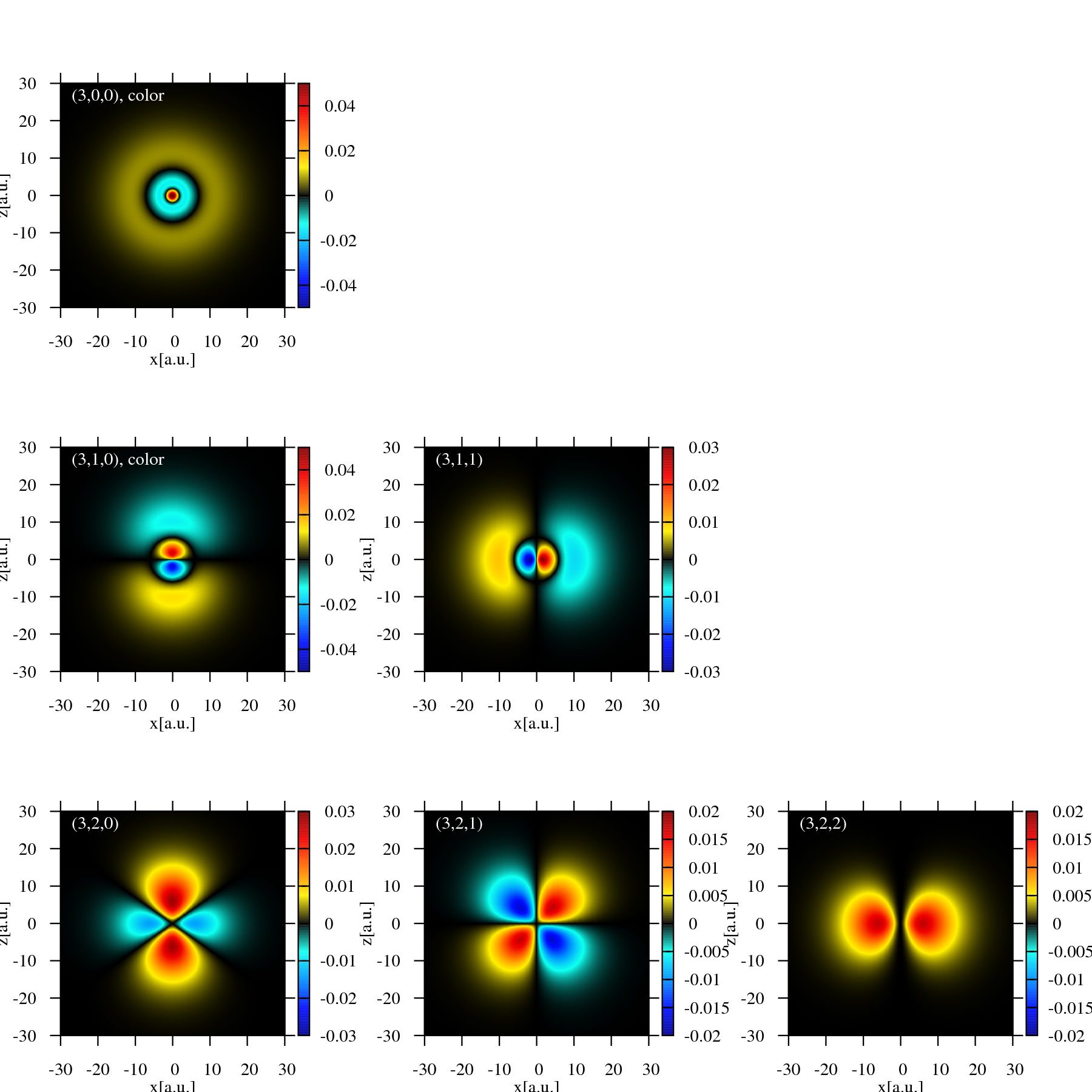
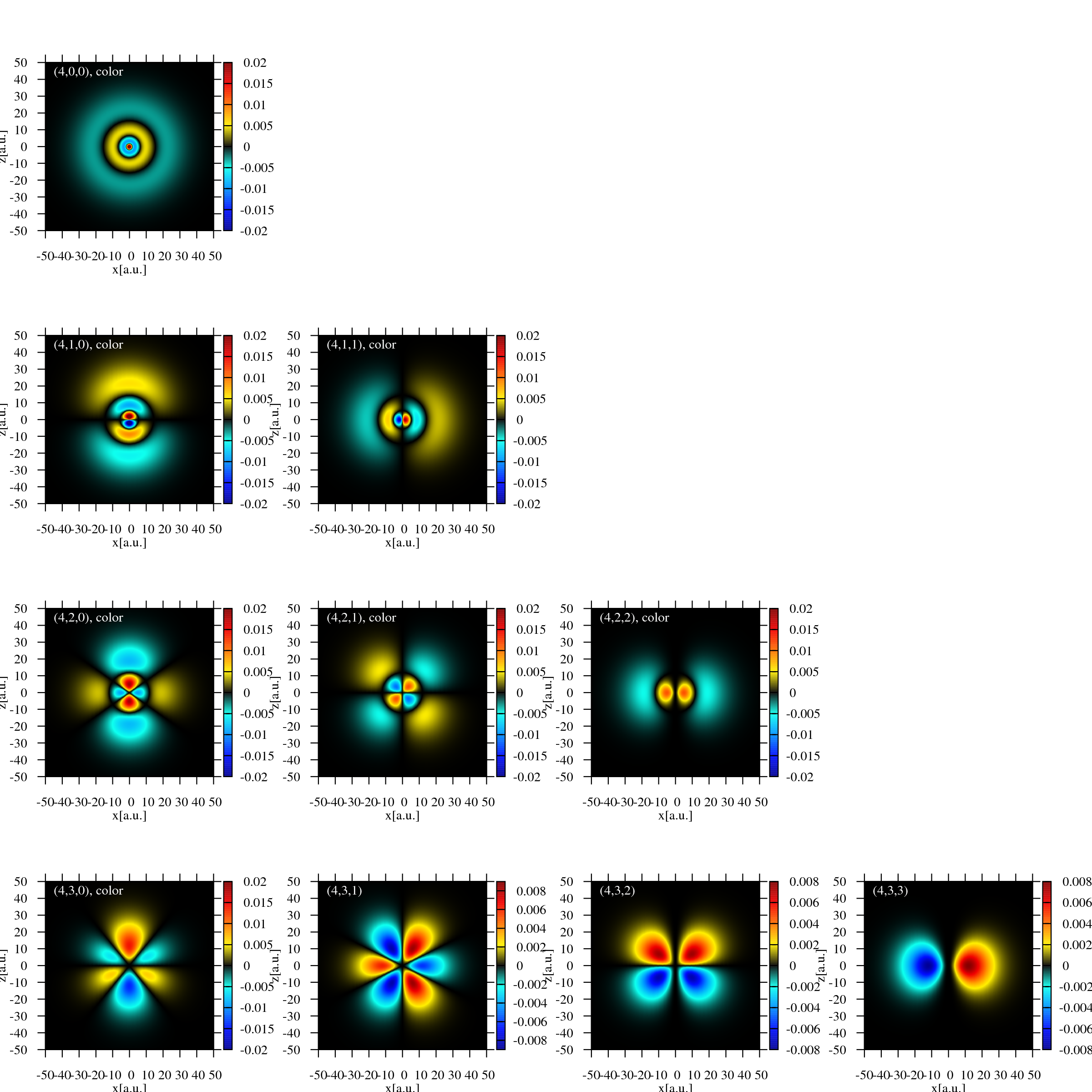
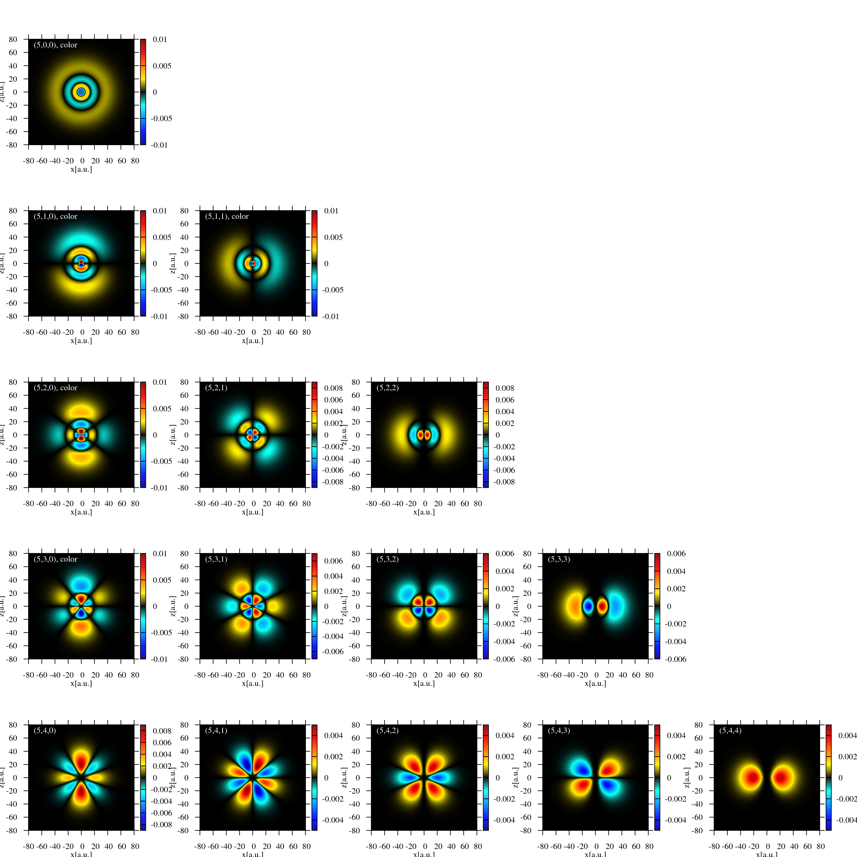
”color”と書いてあるのは、波動関数の形がはっきり映るようにカラーバーの範囲を調整したものです。
なので、色が飽和しているところはそのカラーバーの範囲で表現することはできない領域です。
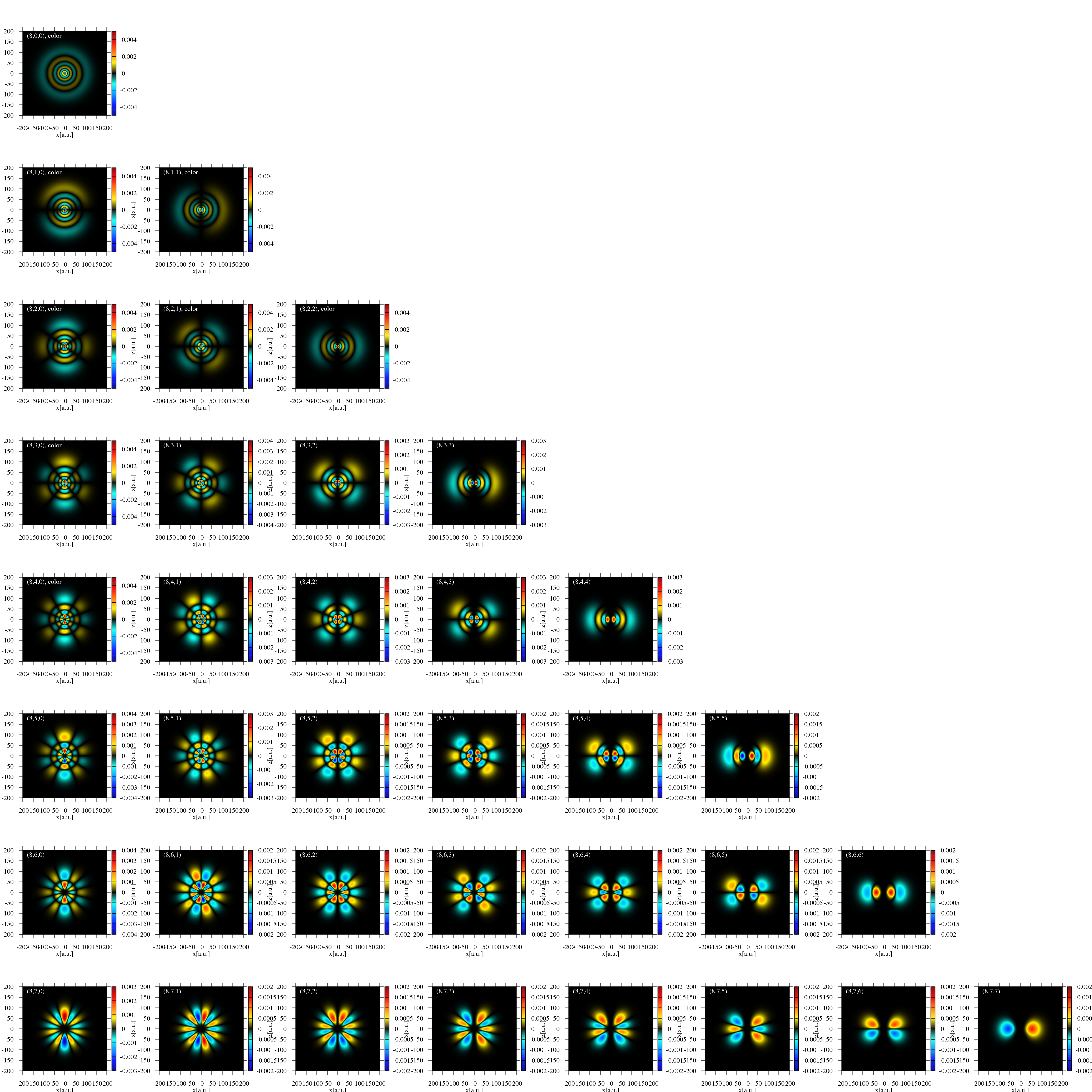
\(n=20\)まで同じような画像を作ったのですが、画像の容量が大きくなりすぎました。
なので、見たい方は以下のリンクから元ファイルをダウンロードしてください。
\(n=1\) Hatomc_n1.png(48KB)
\(n=2\) Hatomc_n2.png(223KB)
\(n=3\) Hatomc_n3.png(612KB)
\(n=4\) Hatomc_n4.png(1MB)
\(n=5\) Hatomc_n5.png(2MB)
\(n=6\) Hatomc_n6.png(3MB)
\(n=7\) Hatomc_n7.png(4MB)
\(n=8\) Hatomc_n8.png(3MB)
\(n=9\) Hatomc_n9.png(6MB)
\(n=10\) Hatomc_n10.png(6MB)
\(n=11\) Hatomc_n11.png(9MB)
\(n=12\) Hatomc_n12.png(9MB)
\(n=13\) Hatomc_n13.png(10MB)
\(n=14\) Hatomc_n14.png(14MB)
\(n=15\) Hatomc_n15.png(15MB)
\(n=16\) Hatomc_n16.png(16MB)
\(n=17\) Hatomc_n17.png(18MB)
\(n=18\) Hatomc_n18.png(19MB)
\(n=19\) Hatomc_n19.png(21MB)
\(n=20\) Hatomc_n20.png(21MB)
n=1~n=20までのファイル hatom.zip(164MB)
例えば、n=13, n=20はこんな感じです(荒くしてます)。
特殊関数に関するプログラミングは特殊関数へ。
How to plot in gnuplot?
Just for note for myself.
You need 2 files which named : multi.plt and atommulti.plt
Before ploting, you must make directory “dat” and move every data files to “dat”.
and in gnuplot, type
then, you can get figure.
multi.plt
atommulti.plt
参考
[1]ラゲール陪多項式\(L_m^{(\alpha)}(x)\)
-
定義域
\(\;\;\;\;
0 \lt x \lt \infty
\) -
微分方程式
\(\;\;\;\;
\displaystyle
\left[x\frac{d^2}{dx^2}+(\alpha+1-x)\frac{d}{dx}+n\right]L_m^{(\alpha)}(x)=0
\) -
具体例
\(\;\;\;\;
\begin{align}
& L^{(0)}_0(x)=1 \\
& L^{(0)}_1(x)=-x+1 \\
& L^{(0)}_2(x)=\frac{1}{2}(x^2-4x+2) \\
& L^{(0)}_3(x)=\frac{1}{6}(-x^3+9x^2-18x+6) \\
& L^{(1)}_0(x)=1 \\
& L^{(1)}_1(x)=-x+2 \\
& L^{(1)}_2(x)=\frac{1}{2}\left(x^2-6x+6\right) \\
& L^{(1)}_3(x)=\frac{1}{6}\left(-x^3+12x^2-36x+24\right)
\end{align}
\) -
漸化式
\(\;\;\;\;
\begin{align}
L_n^{(\alpha)}(x)&=\binom{n+\alpha}{n}a_0(x) \\
&\hspace{1em}a_{m-1}(x)=1-\frac{n-m+1}{m(\alpha+m)}\cdot x\cdot a_m(x) \\
&\hspace{5em}(m=n,n-1,n-2,\cdots,1,\;\;a_n(x)=1)
\end{align}
\)
[3]
1階微分
\(\;\;\;\;
\begin{align}
\frac{d}{dx}L_n^{(\alpha)}(x)=-L_{n-1}^{(\alpha+1)}(x)
\end{align}
\)
2階微分
\(\;\;\;\;
\begin{align}
\frac{d^2}{dx^2}L_n^{(\alpha)}(x)=L_{n-2}^{(\alpha+2)}(x)
\end{align}
\) -
直交性
\(\;\;\;\;
\displaystyle
\int_{0}^{\infty} e^{-x}x^{\alpha}L^{(\alpha)}_n(x)L^{(\alpha)}_{n’}(x) dx =\frac{\Gamma(\alpha+n+1)}{n!}\delta_{n,n’},\;\;(\alpha>-1)
\)
[2]球面調和関数\(Y_{l,m}(\theta,\varphi)\)
ルジャンドル多項式(\(P_l^m(x)\),[3])を用いて
\(
Y_{l,m}(\theta,\varphi)=(-1)^{(m+|m|)/2}\sqrt{\frac{2l+1}{4\pi}\frac{(l-|m|)!}{(l+|m|)!}}P_l^{|m|}(\cos\theta)e^{im\phi}
\)
[3]ルジャンドル陪多項式\(P_l^m(x)\)
-
定義域
\(\;\;\;\;
1 \lt x \lt -1
\) -
微分方程式
\(\;\;\;\;
\displaystyle (1-x^2)\frac{d^2}{dx^2}P_l^m(x)-2x\frac{d}{dx}P_l^m(x)+\left[l(l+1)-\frac{m^2}{1-x^2}\right]P_l^m(x)=0
\) -
具体例
\(\;\;\;\;
\begin{align}
& P_0^0(x)=1 \\
& P_{1}^{-1}(x)=\frac{1}{2}(1-x^2)^{1/2} \\
& P_{1}^{0}(x)=x \\
& P_{1}^{1}(x)=-(1-x^2)^{1/2} \\
& P_{2}^{-2}(x)=\frac{1}{8}(1-x^2) \\
& P_{2}^{-1}(x)=\frac{1}{2}x(1-x^2)^{1/2} \\
& P_{2}^{0}(x)=\frac{1}{2}(3x^2-1) \\
& P_{2}^{1}(x)=-3(1-x^2)^{1/2} \\
& P_{2}^{2}(x)=3(1-x^2)
\end{align}
\) -
漸化式
用いている式
\(\;\;\;\;
\begin{align}
& P_{|m|}^{|m|}(x)=(-1)^{|m|}(2|m|-1)!!(1-x^2)^{\frac{|m|}{2}} \\
& P_{l}^{-m}(x)=(-1)^m\frac{(l-m)!}{(l+m)!}P_l^m(x) \\
& P_{|m|}^{|m|+1}(x)=(2|m|+1)xP_{|m|}^{|m|}(x) \\
& P_{|m|}^{|m|+q}(x)=\left(\frac{2|m|-1}{q}+2\right)xP_{|m|}^{|m|+q-1}(x)-\left(\frac{2|m|-1}{q}+1\right)P_{|m|}^{|m|+q-2}(x)
\end{align}
\)[1]
1階微分
\(\;\;\;\;
\begin{align}
m=\pm 1&\; \\
&:\hspace{1em} \frac{d}{dx}P_l^m(x)=\frac{lx}{(x^2-1)}P_l^m(x)-\frac{l+m}{(x^2-1)} P_{l-1}^m(x) \\
m\ne\pm 1\; \\
&:\hspace{1em} \frac{d}{dx}P_l^m(x)=c_{2}P^{m+2}_{l-1}(x)+c_0 P^{m}_{l-1}(x)+c_{-2} P^{m-2}_{l-1}(x) \\
&\hspace{1em} c_{2}=\frac{1}{4(m+1)}\\
&\hspace{1em} c_{0}=\frac{l+m}{2}\left(1+\frac{l}{1-m^2}\right)\\
&\hspace{1em} c_{-2}=-\frac{(l+m)(l+m-1)(l+m-2)(l-m+1)}{4(m-1)}
\end{align}
\)
※\(m=\pm 1\)の時、\(x=\pm 1\)で発散します。
2階微分
\(\;\;\;\;
\begin{align}
m=\pm 1,\pm 3&\; \\
&:\hspace{1em} \frac{d^2}{dx^2}P_l^m(x)=\frac{1}{1-x^2}\left[2x\frac{dP_l^m(x)}{dx}+\frac{(l+1)(l+m)}{2l+1}\frac{dP_{l-1}^m(x)}{dx}-\frac{l(l-m+1)}{2l+1}\frac{dP_{l+1}^m(x)}{dx}\right] \\
m\ne\pm 1,\pm 3&\; \\
&:\hspace{1em} \frac{d^2}{dx^2}P_l^m(x)=c_{2}\frac{dP^{m+2}_{l-1}(x)}{dx}+c_0 \frac{dP^{m}_{l-1}(x)}{dx}+c_{-2} \frac{dP^{m-2}_{l-1}(x)}{dx}
\end{align}
\)
※\(m=\pm 1,\pm 3\)の時、\(x=\pm 1\)で発散します。 -
直交性
\(l\)に対する直交性
\(\;\;\;\;
\displaystyle
\int_{-1}^{1} P_{m}^{l}(x)P_{m}^{l’}(x) dx =\frac{2}{2l+1}\cdot \frac{(l+m)!}{(l-m)!}\delta_{l,l’}
\)
[3] Abramowitz & Stegun (1965), ISBN 978-0486612720 (Numerical Method, 22.18, Page 789)
[4] Abramowitz & Stegun (1965), ISBN 978-0486612720 (Numerical Method, 22.2, Page 774,775)
