
多項式補間です。
- Cubic補間 (1次元) \(O(h^4)\)
- Bicubic補間 (2次元) \(O(h^4)\)
- 補間 (2次元) \(O(h^2)\)
- 参考文献
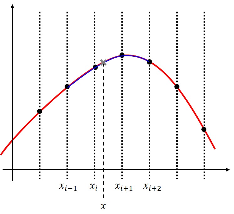
Cubic補間 (1次元)
4点を厳密に通る3次多項式によって関数を補間します。
概要は以下の図の通りです。
補間したい点よりも小さいデータ点を2点、大きいデータ点を2点使って補間します。
いわば小さい区間で区切ったラグランジュ補間です。
補間は,既知の係数\(a_{i}\)を用いて関数
\(\displaystyle
g(x)=\sum_{i=0}^{3}a_{i}x^i
\)
誤差は\(O(h^4)\)です。
Fortranプログラムはこちら。
program main
implicit none
integer::i,N,M
double precision::x,f,df,df2,s
double precision,allocatable::xdata(:),fdata(:)
double precision::pi=dacos(-1d0)
double precision,external::cubic
N=30
M=100
allocate(xdata(0:N),fdata(0:N))
xdata=0d0
fdata=0d0
do i=0,N
xdata(i)=dble(i)*0.1d0*pi
fdata(i)=sin(xdata(i))
write(10,*)xdata(i),fdata(i)
enddo
! Cubic-spline interpolation given position as point
do i=0,M
x=dble(i)*0.03d0*pi-1d0
write(11,'(2e20.7e2)')x,cubic(x,N,xdata,fdata)
enddo
stop
end program main
double precision function cubic(x,N,x0,f0)
implicit none
integer,intent(in)::N
double precision,intent(in)::x,f0(0:N),x0(0:N)
integer::i,i0,i1,i2,i3
double precision::tx
double precision::a,b,c,d,p,q,r,s,t,u
tx = x-x0(0)
i1 = 0
do i=1,N-2
tx = x-x0(i)
if(tx.gt.0d0)then
i1 = i
else
exit
endif
enddo
if(i1.eq.0)i1=1
i0=i1-1
i2=i1+1
i3=i1+2
a = x-x0(i0)
b = x-x0(i1)
c = x-x0(i2)
d = x-x0(i3)
p = x0(i1)-x0(i0)
q = x0(i2)-x0(i1)
r = x0(i3)-x0(i2)
s = x0(i2)-x0(i0)
t = x0(i3)-x0(i1)
u = x0(i3)-x0(i0)
cubic = a*c*( d*f0(i1)/(p*q) + b*f0(i3)/(u*r) )/t &
- b*d*( c*f0(i0)/(p*u) + a*f0(i2)/(q*r) )/s
return
end function cubic
implicit none
integer::i,N,M
double precision::x,f,df,df2,s
double precision,allocatable::xdata(:),fdata(:)
double precision::pi=dacos(-1d0)
double precision,external::cubic
N=30
M=100
allocate(xdata(0:N),fdata(0:N))
xdata=0d0
fdata=0d0
do i=0,N
xdata(i)=dble(i)*0.1d0*pi
fdata(i)=sin(xdata(i))
write(10,*)xdata(i),fdata(i)
enddo
! Cubic-spline interpolation given position as point
do i=0,M
x=dble(i)*0.03d0*pi-1d0
write(11,'(2e20.7e2)')x,cubic(x,N,xdata,fdata)
enddo
stop
end program main
double precision function cubic(x,N,x0,f0)
implicit none
integer,intent(in)::N
double precision,intent(in)::x,f0(0:N),x0(0:N)
integer::i,i0,i1,i2,i3
double precision::tx
double precision::a,b,c,d,p,q,r,s,t,u
tx = x-x0(0)
i1 = 0
do i=1,N-2
tx = x-x0(i)
if(tx.gt.0d0)then
i1 = i
else
exit
endif
enddo
if(i1.eq.0)i1=1
i0=i1-1
i2=i1+1
i3=i1+2
a = x-x0(i0)
b = x-x0(i1)
c = x-x0(i2)
d = x-x0(i3)
p = x0(i1)-x0(i0)
q = x0(i2)-x0(i1)
r = x0(i3)-x0(i2)
s = x0(i2)-x0(i0)
t = x0(i3)-x0(i1)
u = x0(i3)-x0(i0)
cubic = a*c*( d*f0(i1)/(p*q) + b*f0(i3)/(u*r) )/t &
- b*d*( c*f0(i0)/(p*u) + a*f0(i2)/(q*r) )/s
return
end function cubic
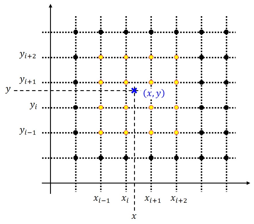
Bicubic補間 (2次元)
16点を厳密に通る多項式によって関数を補間します。
補間したい点を囲むように存在する16点を用いて補間します。
補間は,既知の係数\(a_{i,j}\)を用いて関数
\(\displaystyle
g(x,y)=\sum_{i=0}^{3}\sum_{j=0}^{3}a_{i,j}x^i y^j
\)
によって行います[1]。誤差は\(O(h^4)\)です。
Fortranプログラムはこちら。
program main
implicit none
integer::i,j
integer::Nx,Ny
double precision::x,y
double precision::xa,xb,ya,yb
double precision,allocatable::x0(:),y0(:),z0(:,:)
double precision,external::f,ip16
Nx=20
Ny=20
allocate(x0(0:Nx), y0(0:Ny), z0(0:Nx,0:Ny))
xa=-3d0
xb= 3d0
ya=-3d0
yb= 3d0
! generate references points
do i=0,Nx
x0(i)=dble(i)*(xb-xa)/Nx+xa
enddo
do j=0,Ny
y0(j)=dble(j)*(yb-ya)/Ny+ya
enddo
do i=0,Nx
do j=0,Ny
z0(i,j)=f(x0(i),y0(j))
write(10,*)x0(i),y0(j),z0(i,j)
enddo
write(10,*)
enddo
! Return interpolated results
do i=0,50
do j=0,50
x=i*0.03d0-1d0
y=j*0.03d0-1d0
write(11,*)x,y,ip16(x,y,Nx,Ny,x0,y0,z0)
enddo
write(11,*)
enddo
stop
end program main
function f(x,y)
implicit none
double precision::f
double precision,intent(in)::x,y
f=x*y*exp(-x*x-y*y)
return
end function f
double precision function ip16(x,y,Nx,Ny,x0,y0,z0)
implicit none
integer,intent(in)::Nx,Ny
double precision,intent(in)::x,y,x0(0:Nx),y0(0:Ny),z0(0:Nx,0:Ny)
!
! Bicubic interpolation
! x0,y0 are sorted by ascending order,
! suppose x0 & y0 are equal interval.
! z0(x0,y0)
!
integer::i,j
integer::i0,i1,i2,i3
integer::j0,j1,j2,j3
double precision::tx,u,u2,u3
double precision::ty,v,v2,v3
double precision::a00,a01,a02,a03,a10,a11,a12,a13
double precision::a20,a21,a22,a23,a30,a31,a32,a33
double precision::p(0:3,0:3)
if(Nx.le.3.or.Ny.le.3)then
write(6,*)" *** Error at ip16"
stop
endif
tx = x-x0(0)
i1 = 0
do i=1,Nx-2
tx = x-x0(i)
if(tx.gt.0d0)then
i1 = i
else
exit
endif
enddo
if(i1.eq.0)i1=1
i0=i1-1
i2=i1+1
i3=i1+2
ty = y-y0(0)
j1 = 0
do j=1,Ny-2
ty = y-y0(j)
if(ty.gt.0d0)then
j1 = j
else
exit
endif
enddo
if(j1.eq.0)j1=1
j0=j1-1
j2=j1+1
j3=j1+2
p(0,0) = z0(i0,j0)
p(0,1) = z0(i0,j1)
p(0,2) = z0(i0,j2)
p(0,3) = z0(i0,j3)
p(1,0) = z0(i1,j0)
p(1,1) = z0(i1,j1)
p(1,2) = z0(i1,j2)
p(1,3) = z0(i1,j3)
p(2,0) = z0(i2,j0)
p(2,1) = z0(i2,j1)
p(2,2) = z0(i2,j2)
p(2,3) = z0(i2,j3)
p(3,0) = z0(i3,j0)
p(3,1) = z0(i3,j1)
p(3,2) = z0(i3,j2)
p(3,3) = z0(i3,j3)
a00 = p(1,1)
a01 = -0.5d0*p(1,0) + 0.5d0*p(1,2)
a02 = p(1,0) - 2.5d0*p(1,1) + 2*p(1,2) - 0.5d0*p(1,3)
a03 = -0.50d0*p(1,0) + 1.50d0*p(1,1) - 1.50d0*p(1,2) + 0.5d0*p(1,3)
a10 = -0.50d0*p(0,1) + 0.50d0*p(2,1)
a11 = 0.25d0*p(0,0) - 0.25d0*p(0,2) - 0.25d0*p(2,0) + 0.25d0*p(2,2)
a12 = -0.50d0*p(0,0) + 1.25d0*p(0,1) - p(0,2) + 0.25d0*p(0,3) &
+ 0.50d0*p(2,0) - 1.25d0*p(2,1) + p(2,2) - 0.25d0*p(2,3)
a13 = 0.25d0*p(0,0) - 0.75d0*p(0,1) + 0.75d0*p(0,2) - 0.25d0*p(0,3) &
- 0.25d0*p(2,0) + 0.75d0*p(2,1) - 0.75d0*p(2,2) + 0.25d0*p(2,3)
a20 = p(0,1) - 2.5d0*p(1,1) + 2.d0*p(2,1) - 0.5d0*p(3,1)
a21 = -0.50d0*p(0,0) + 0.5d0*p(0,2) + 1.25d0*p(1,0) - 1.25d0*p(1,2) &
- p(2,0) + p(2,2) + 0.25d0*p(3,0) - 0.25d0*p(3,2)
a22 = p(0,0) - 2.5d0*p(0,1) + 2.0d0*p(0,2) - 0.50d0*p(0,3) &
- 2.5d0*p(1,0) + 6.25d0*p(1,1) - 5d0*p(1,2) + 1.25d0*p(1,3) &
+ 2.0d0*p(2,0) - 5.0d0*p(2,1) + 4d0*p(2,2) - p(2,3) &
- 0.50d0*p(3,0) + 1.25d0*p(3,1) - p(3,2) + 0.25d0*p(3,3)
a23 = -0.50d0*p(0,0) + 1.50d0*p(0,1) - 1.50d0*p(0,2) + 0.5d0*p(0,3) &
+ 1.25d0*p(1,0) - 3.75d0*p(1,1) + 3.75d0*p(1,2) - 1.25d0*p(1,3) &
- p(2,0) + 3*p(2,1) - 3*p(2,2) + p(2,3) &
+ 0.25d0*p(3,0) - 0.75d0*p(3,1) + 0.75d0*p(3,2) - 0.25d0*p(3,3)
a30 = -0.50d0*p(0,1) + 1.50d0*p(1,1) - 1.50d0*p(2,1) + 0.5d0*p(3,1)
a31 = 0.25d0*p(0,0) - 0.25d0*p(0,2) - 0.75d0*p(1,0) + 0.75d0*p(1,2) &
+ 0.75d0*p(2,0) - 0.75d0*p(2,2) - 0.25d0*p(3,0) + 0.25d0*p(3,2)
a32 = -0.50d0*p(0,0) + 1.25d0*p(0,1) - p(0,2) + 0.25d0*p(0,3) &
+ 1.50d0*p(1,0) - 3.75d0*p(1,1) + 3*p(1,2) - 0.75d0*p(1,3) &
- 1.50d0*p(2,0) + 3.75d0*p(2,1) - 3*p(2,2) + 0.75d0*p(2,3) &
+ 0.50d0*p(3,0) - 1.25d0*p(3,1) + p(3,2) - 0.25d0*p(3,3)
a33 = 0.25d0*p(0,0) - 0.75d0*p(0,1) + 0.75d0*p(0,2) - 0.25d0*p(0,3) &
- 0.75d0*p(1,0) + 2.25d0*p(1,1) - 2.25d0*p(1,2) + 0.75d0*p(1,3) &
+ 0.75d0*p(2,0) - 2.25d0*p(2,1) + 2.25d0*p(2,2) - 0.75d0*p(2,3) &
- 0.25d0*p(3,0) + 0.75d0*p(3,1) - 0.75d0*p(3,2) + 0.25d0*p(3,3)
! Parallel translation u,v [0:1]
u = (x-x0(i1))/(x0(i2)-x0(i1))
v = (y-y0(j1))/(y0(j2)-y0(j1))
u2 = u*u
u3 = u2*u
v2 = v*v
v3 = v2*v
ip16= (a00 + a01 * v + a02 * v2 + a03 * v3) &
+ (a10 + a11 * v + a12 * v2 + a13 * v3) * u &
+ (a20 + a21 * v + a22 * v2 + a23 * v3) * u2 &
+ (a30 + a31 * v + a32 * v2 + a33 * v3) * u3
return
end function ip16
implicit none
integer::i,j
integer::Nx,Ny
double precision::x,y
double precision::xa,xb,ya,yb
double precision,allocatable::x0(:),y0(:),z0(:,:)
double precision,external::f,ip16
Nx=20
Ny=20
allocate(x0(0:Nx), y0(0:Ny), z0(0:Nx,0:Ny))
xa=-3d0
xb= 3d0
ya=-3d0
yb= 3d0
! generate references points
do i=0,Nx
x0(i)=dble(i)*(xb-xa)/Nx+xa
enddo
do j=0,Ny
y0(j)=dble(j)*(yb-ya)/Ny+ya
enddo
do i=0,Nx
do j=0,Ny
z0(i,j)=f(x0(i),y0(j))
write(10,*)x0(i),y0(j),z0(i,j)
enddo
write(10,*)
enddo
! Return interpolated results
do i=0,50
do j=0,50
x=i*0.03d0-1d0
y=j*0.03d0-1d0
write(11,*)x,y,ip16(x,y,Nx,Ny,x0,y0,z0)
enddo
write(11,*)
enddo
stop
end program main
function f(x,y)
implicit none
double precision::f
double precision,intent(in)::x,y
f=x*y*exp(-x*x-y*y)
return
end function f
double precision function ip16(x,y,Nx,Ny,x0,y0,z0)
implicit none
integer,intent(in)::Nx,Ny
double precision,intent(in)::x,y,x0(0:Nx),y0(0:Ny),z0(0:Nx,0:Ny)
!
! Bicubic interpolation
! x0,y0 are sorted by ascending order,
! suppose x0 & y0 are equal interval.
! z0(x0,y0)
!
integer::i,j
integer::i0,i1,i2,i3
integer::j0,j1,j2,j3
double precision::tx,u,u2,u3
double precision::ty,v,v2,v3
double precision::a00,a01,a02,a03,a10,a11,a12,a13
double precision::a20,a21,a22,a23,a30,a31,a32,a33
double precision::p(0:3,0:3)
if(Nx.le.3.or.Ny.le.3)then
write(6,*)" *** Error at ip16"
stop
endif
tx = x-x0(0)
i1 = 0
do i=1,Nx-2
tx = x-x0(i)
if(tx.gt.0d0)then
i1 = i
else
exit
endif
enddo
if(i1.eq.0)i1=1
i0=i1-1
i2=i1+1
i3=i1+2
ty = y-y0(0)
j1 = 0
do j=1,Ny-2
ty = y-y0(j)
if(ty.gt.0d0)then
j1 = j
else
exit
endif
enddo
if(j1.eq.0)j1=1
j0=j1-1
j2=j1+1
j3=j1+2
p(0,0) = z0(i0,j0)
p(0,1) = z0(i0,j1)
p(0,2) = z0(i0,j2)
p(0,3) = z0(i0,j3)
p(1,0) = z0(i1,j0)
p(1,1) = z0(i1,j1)
p(1,2) = z0(i1,j2)
p(1,3) = z0(i1,j3)
p(2,0) = z0(i2,j0)
p(2,1) = z0(i2,j1)
p(2,2) = z0(i2,j2)
p(2,3) = z0(i2,j3)
p(3,0) = z0(i3,j0)
p(3,1) = z0(i3,j1)
p(3,2) = z0(i3,j2)
p(3,3) = z0(i3,j3)
a00 = p(1,1)
a01 = -0.5d0*p(1,0) + 0.5d0*p(1,2)
a02 = p(1,0) - 2.5d0*p(1,1) + 2*p(1,2) - 0.5d0*p(1,3)
a03 = -0.50d0*p(1,0) + 1.50d0*p(1,1) - 1.50d0*p(1,2) + 0.5d0*p(1,3)
a10 = -0.50d0*p(0,1) + 0.50d0*p(2,1)
a11 = 0.25d0*p(0,0) - 0.25d0*p(0,2) - 0.25d0*p(2,0) + 0.25d0*p(2,2)
a12 = -0.50d0*p(0,0) + 1.25d0*p(0,1) - p(0,2) + 0.25d0*p(0,3) &
+ 0.50d0*p(2,0) - 1.25d0*p(2,1) + p(2,2) - 0.25d0*p(2,3)
a13 = 0.25d0*p(0,0) - 0.75d0*p(0,1) + 0.75d0*p(0,2) - 0.25d0*p(0,3) &
- 0.25d0*p(2,0) + 0.75d0*p(2,1) - 0.75d0*p(2,2) + 0.25d0*p(2,3)
a20 = p(0,1) - 2.5d0*p(1,1) + 2.d0*p(2,1) - 0.5d0*p(3,1)
a21 = -0.50d0*p(0,0) + 0.5d0*p(0,2) + 1.25d0*p(1,0) - 1.25d0*p(1,2) &
- p(2,0) + p(2,2) + 0.25d0*p(3,0) - 0.25d0*p(3,2)
a22 = p(0,0) - 2.5d0*p(0,1) + 2.0d0*p(0,2) - 0.50d0*p(0,3) &
- 2.5d0*p(1,0) + 6.25d0*p(1,1) - 5d0*p(1,2) + 1.25d0*p(1,3) &
+ 2.0d0*p(2,0) - 5.0d0*p(2,1) + 4d0*p(2,2) - p(2,3) &
- 0.50d0*p(3,0) + 1.25d0*p(3,1) - p(3,2) + 0.25d0*p(3,3)
a23 = -0.50d0*p(0,0) + 1.50d0*p(0,1) - 1.50d0*p(0,2) + 0.5d0*p(0,3) &
+ 1.25d0*p(1,0) - 3.75d0*p(1,1) + 3.75d0*p(1,2) - 1.25d0*p(1,3) &
- p(2,0) + 3*p(2,1) - 3*p(2,2) + p(2,3) &
+ 0.25d0*p(3,0) - 0.75d0*p(3,1) + 0.75d0*p(3,2) - 0.25d0*p(3,3)
a30 = -0.50d0*p(0,1) + 1.50d0*p(1,1) - 1.50d0*p(2,1) + 0.5d0*p(3,1)
a31 = 0.25d0*p(0,0) - 0.25d0*p(0,2) - 0.75d0*p(1,0) + 0.75d0*p(1,2) &
+ 0.75d0*p(2,0) - 0.75d0*p(2,2) - 0.25d0*p(3,0) + 0.25d0*p(3,2)
a32 = -0.50d0*p(0,0) + 1.25d0*p(0,1) - p(0,2) + 0.25d0*p(0,3) &
+ 1.50d0*p(1,0) - 3.75d0*p(1,1) + 3*p(1,2) - 0.75d0*p(1,3) &
- 1.50d0*p(2,0) + 3.75d0*p(2,1) - 3*p(2,2) + 0.75d0*p(2,3) &
+ 0.50d0*p(3,0) - 1.25d0*p(3,1) + p(3,2) - 0.25d0*p(3,3)
a33 = 0.25d0*p(0,0) - 0.75d0*p(0,1) + 0.75d0*p(0,2) - 0.25d0*p(0,3) &
- 0.75d0*p(1,0) + 2.25d0*p(1,1) - 2.25d0*p(1,2) + 0.75d0*p(1,3) &
+ 0.75d0*p(2,0) - 2.25d0*p(2,1) + 2.25d0*p(2,2) - 0.75d0*p(2,3) &
- 0.25d0*p(3,0) + 0.75d0*p(3,1) - 0.75d0*p(3,2) + 0.25d0*p(3,3)
! Parallel translation u,v [0:1]
u = (x-x0(i1))/(x0(i2)-x0(i1))
v = (y-y0(j1))/(y0(j2)-y0(j1))
u2 = u*u
u3 = u2*u
v2 = v*v
v3 = v2*v
ip16= (a00 + a01 * v + a02 * v2 + a03 * v3) &
+ (a10 + a11 * v + a12 * v2 + a13 * v3) * u &
+ (a20 + a21 * v + a22 * v2 + a23 * v3) * u2 &
+ (a30 + a31 * v + a32 * v2 + a33 * v3) * u3
return
end function ip16
補間 (2次元)
Bicubic補間の低次元バージョンです。
補間したい点を囲むように存在する4点を用いて補間します。
一応Four point Formulaと名づけられています[2]。
補間は,既知の係数\(a_{i,j}\)を用いて関数
\(\displaystyle
g(x,y)=\sum_{i=0}^{1}\sum_{j=0}^{1}a_{i,j}x^i y^j
\)
によって行います[2]。誤差は\(O(h^2)\)です。
function ip4(x,y,Nx,Ny,x0,y0,z0)
implicit none
integer,intent(in)::Nx,Ny
double precision,intent(in)::x,y,x0(1:Nx),y0(1:Ny),z0(1:Nx,1:Ny)
double precision::ip4
!
! 2D Interpolation, 4-point formula,
! xy equal distance grid
!
integer::i,ix0,ix1,iy0,iy1
double precision::tx,ty,dx,dy,p,q
tx=1d100
ix0=1
do i=2,Nx
if(abs(x-x0(i)).le.tx)then
tx=abs(x-x0(i))
ix0=i
endif
enddo
tx=1d100
ix1=1
do i=2,Nx
if(i.ne.ix0)then
if(abs(x-x0(i)).le.tx)then
tx=abs(x-x0(i))
ix1=i
endif
endif
enddo
ty=1d100
iy0=1
do i=2,Ny
if(abs(y-y0(i)).le.ty)then
ty=abs(y-y0(i))
iy0=i
endif
enddo
ty=1d100
iy1=1
do i=2,Ny
if(i.ne.iy0)then
if(abs(y-y0(i)).le.ty)then
ty=abs(y-y0(i))
iy1=i
endif
endif
enddo
dx=x0(ix1)-x0(ix0)
dy=y0(iy1)-y0(iy0)
p=(x-x0(ix0))/dx
q=(y-y0(iy0))/dy
ip4=(1d0-p)*(1d0-q)*z0(ix0,iy0) &
+p*(1d0-q)*z0(ix1,iy0) &
+(1d0-p)*q*z0(ix0,iy1) &
+p*q*z0(ix1,iy1)
return
end function ip4
参考文献
[1]Cubic interpolation
[2]Abramowitz and Stegun.
Handbook of Mathematical Functions.