sikino のすべての投稿

ファイル読み込み

ファイルの読み込みに関するサブルーチンを記述します。

 do i=1,4
     do j=1,83
        write(30,*)i,j,i*j
     end do
     write(30,*)
  end do

によってファイル”fort.30″が作られたとします。
今、fort.30を読み込んで
“i”の数”4”

“j”の数”83″
を取り出したいとします。

read文を使って読み込みますが、そのまま読み込むと空白部分を読み込んだり、読み込まないだったりします。
ここでは上のdoループによって作られたファイルの場合に使えるものを想定します。

ここでは、
大きな塊を表す数である”4″をblock,
塊の中の要素数を表す”83″をelement
と呼ぶことにします。

この問題を解く戦略は、ファイルを読み込む2種類の方法です。
1つは本当の行数(空行含む)を数え、もう1つは空行を飛ばして読み込む方法です。
本当の行数を数えるサブルーチンは下の”linecount”
であり、
空行を読み飛ばして行数を数えるサブルーチンは下の”linecount_eff”
です。
この二つと、一番下の行に追加される余分な1行を対処するために”breaklinecheck”というルーチンを使います。

これによってblockとelementを出力するサブルーチン”blockelement”を作っています。

下のプログラムを実行すると

$ gfortran main.f90
$ ./a.out
 ===Apply for fortran file will done===
 Nblock     ::         4
 Nelement   ::        83

という結果が得られるかと思います。

program main
  !developer => sikinote
  !date      => 2015/03/31
  implicit none
  integer::NBlock,Nelement
  character(48)::filename
 
  filename='./fort.30'
  call blockelement(filename,Nblock,Nelement)

  write(6,'(A,i10)')" Nblock     ::",Nblock
  write(6,'(A,i10)')" Nelement   ::",Nelement

  stop
end program
!===================================
   
subroutine blockelement(filename,Nblock,Nelement)
  !developer => sikino
  !date      => 2015/03/31
  implicit none
  character(*),intent(in)::filename
  integer,intent(out)::Nblock,Nelement
  integer::c1,c2
 
  call linecount(c1,filename)
  call linecount_eff(c2,filename)
  call breaklinecheck(c1,c2)
  Nblock=c1-c2+1
  Nelement=c2/Nblock
 
  return
end subroutine blockelement
!------------------------------
subroutine linecount(c,filename)
  implicit none
  integer,intent(out)::c
  character(*),intent(in)::filename

  integer::ier
  character(len_trim(filename))::fname
 
  fname=trim(filename)
  c=0
  open(100,file=fname,status='old',iostat=ier,err=990)
  do while(.true.)
     read(100,*,end=999)
     c=c+1
  enddo
999 continue
  close(100)
   
  return
!+-----------------------+
990 write(6,'(A)')"!!!!==error when open file",trim(fname),"info-->",ier
  write(6,*)"======program stop at linecount"
  stop

end subroutine linecount
!--------------------------------
subroutine linecount_eff(c,filename)
  implicit none
  integer,intent(out)::c
  character(*),intent(in)::filename

  integer::ier
  character(100)::cc
  character(len_trim(filename))::fname
 
  fname=trim(filename)

  c=0
  open(100,file=fname,status='old',iostat=ier,err=990)
  do while(.true.)
     read(100,*,end=998)cc
     if(len_trim(cc).gt.0)c=c+1
  enddo

998 continue
  close(100)
  return

990 write(6,'(A)')"!!!!==error when open file",trim(fname),"info==>",ier
  write(6,*)"======program stop at linecount_eff"
  stop

end subroutine linecount_eff
!-------------------------------------
subroutine breaklinecheck(c1,c2)
  implicit none
  integer,intent(inout)::c1
  integer,intent(in)::c2
  integer::Nb
 
  Nb=c1-c2+1
  if(Nb.eq.2.or.mod(c2,Nb).ne.0)then
     write(6,*)"===Apply for fortran file will done==="
     c1=c1-1
     Nb=c1-c2+1
     if(mod(c2,Nb).ne.0)then
        write(6,*)"line is different(may be last break)"
        write(6,*)"program stop at subroutine __breaklinecheck__"
        stop
     end if
  endif
 
  return
end subroutine breaklinecheck

データを読み込むには?


さて、ブロックの数と要素の数が上のサブルーチンを使うことにより求められることがわかりました。
実際にデータを配列に代入するためにはどうすればいいんでしょう?
型に応じて使うサブルーチンを変えます。
その手続きは下のモジュールを記述することでokです。これを書いた上で、
メインプログラムを以下のように書きます。そうすれば配列x(,)とy(,)に値がはいります。

program main
  use read1
  implicit none
  integer::NBlock,Nelement,i,j
  character(48)::filename
 
  double precision,allocatable::x(:,:),y(:,:)
 
  filename='./fort.30'
  call blockelement(filename,Nblock,Nelement)

  write(6,'(A,i10)')" Nblock     ::",Nblock
  write(6,'(A,i10)')" Nelement   ::",Nelement
 
  allocate(x(1:Nblock,1:Nelement),y(1:Nblock,1:Nelement))
  call read_filedata(size(y,1),size(y,2),x,y,filename)
 
  do i=1,Nblock
     do j=1,Nelement
        write(11,*)x(i,j),y(i,j)
     enddo
     write(11,*)
  enddo
 
  stop
end program

総称名を用いる場合の手続き(read_filedata())

module read1
  implicit none
  interface read_filedata
     module procedure &
          ! dx1 -> double precision array, x(:)
          ! cy2 -> complex array, y(:,:)
          ! xyy -> coloum of file, | x y y |
          read_dx0_dy1_xy, &
          read_dx0_cy1_xyy, &
          read_dx1_dy1_xy, &
          read_dx1_cy1_xyy, &
          read_dx1_dy2_xy, &
          read_dx1_cy2_xyy, &
          read_dx2_dy2_xy, &
          read_dx2_cy2_xyy
  end interface read_filedata
contains
  subroutine read_dx0_dy1_xy(Ne,y,place,col12)
    integer,intent(in)::Ne,col12
    character(*),intent(in)::place
    double precision,intent(out)::y(1:Ne)

    integer::i,ier
    double precision::a,b
    character(len_trim(place))::fn

    y=0d0
    fn=trim(place)

    open(28,file=fn,status='old',iostat=ier,err=977)
    if(col12.eq.1)then
       do i=1,Ne
          read(28,*)a,b
          y(i)=a
       enddo
    elseif(col12.eq.2)then
       do i=1,Ne
          read(28,*)a,b
          y(i)=b
       enddo
    else
       go to 977
    endif
             
    close(28)
    return

977 write(6,'(3A,i5)')"!!!!==error when open file",trim(fn),"info==>",ier
    write(6,*)"======program stop at read_dx0_dy1_11"
    stop
  end subroutine read_dx0_dy1_xy

  subroutine read_dx0_cy1_xyy(Ne,y,place)
    integer,intent(in)::Ne
    character(*),intent(in)::place
    complex(kind(0d0)),intent(out)::y(1:Ne)

    integer::i,ier
    double precision::a,b,c
    character(len_trim(place))::fn

    y=0d0
    fn=trim(place)

    open(28,file=fn,status='old',iostat=ier,err=977)
    do i=1,Ne
       read(28,*)a,b,c
       y(i)=dcmplx(b,c)
    enddo
    close(28)
    return

977 write(6,'(3A,i5)')"!!!!==error when open file",trim(fn),"info==>",ier
    write(6,*)"======program stop at read_dx0_cy1_xyy"
    stop
  end subroutine read_dx0_cy1_xyy

  subroutine read_dx1_dy1_xy(Ne,x,y,place)
    integer,intent(in)::Ne
    character(*),intent(in)::place
    double precision,intent(out)::x(1:Ne),y(1:Ne)

    character(len_trim(place))::fn
    double precision::a,b
    integer::i,ier

    x=0d0; y=0d0
   
    fn=trim(place)
    open(28,file=trim(fn),status='old',iostat=ier,err=977)
    do i=1,Ne
       read(28,*)a,b
       x(i)=a
       y(i)=b
    enddo
    close(28)
    return

977 write(6,'(3A,i5)')"!!!!==error when open file",trim(fn),"info==>",ier
    write(6,*)"======program stop at read_dx1_dy1_xy"
    stop
  end subroutine read_dx1_dy1_xy
 
  subroutine read_dx1_cy1_xyy(Ne,x,y,place)
    integer,intent(in)::Ne
    character(*),intent(in)::place
    double precision,intent(out)::x(1:Ne)
    complex(kind(0d0)),intent(out)::y(1:Ne)

    integer::i,ier
    double precision::a,b,c
    character(len_trim(place))::fn

    y=0d0
    fn=trim(place)

    open(28,file=fn,status='old',iostat=ier,err=977)
    do i=1,Ne
       read(28,*)a,b,c
       x(i)=a
       y(i)=dcmplx(b,c)
    enddo
    close(28)
    return

977 write(6,'(3A,i5)')"!!!!==error when open file",trim(fn),"info==>",ier
    write(6,*)"======program stop at read_dx1_cy1_xyy"
    stop
  end subroutine read_dx1_cy1_xyy

  subroutine read_dx1_dy2_xy(Nb,Ne,x,y,place)
    integer,intent(in)::Nb,Ne
    double precision,intent(out)::x(1:Ne),y(1:Nb,1:Ne)
    character(*),intent(in)::place
   
    integer::i,j,ier
    character(len_trim(place))::fn
    double precision::a,b
   
    x=0d0; y=0d0
   
    fn=trim(place)
    open(28,file=trim(fn),status='old',iostat=ier,err=977)
    do i=1,Nb
       do j=1,Ne
          read(28,*)a,b
          if(i.eq.1)x(j)=a
          y(i,j)=b
       enddo
    enddo
    close(28)
    return

977 write(6,'(3A,i5)')"!!!!==error when open file",trim(fn),"info==>",ier
    write(6,*)"======program stop at read_dx1_dy2_xy"
    stop
  end subroutine read_dx1_dy2_xy
 
  subroutine read_dx1_cy2_xyy(Nb,Ne,x,y,place)
    integer,intent(in)::Nb,Ne
    double precision,intent(out)::x(1:Ne)
    complex(kind(0d0)),intent(out)::y(1:Nb,1:Ne)
    character(*),intent(in)::place

    integer::i,j,ier
    character(len_trim(place))::fn
    double precision::a,b,c

    x=0d0; y=0d0

    fn=trim(place)
    open(28,file=trim(fn),status='old',iostat=ier,err=977)
    do i=1,Nb
       do j=1,Ne
          read(28,*)a,b,c
          if(i.eq.1)x(j)=a
          y(i,j)=dcmplx(b,c)
       enddo
    enddo
    close(28)
    return

977 write(6,'(3A,i5)')"!!!!==error when open file",trim(fn),"info==>",ier
    write(6,*)"======program stop at read_dx1_cy2_12"
    stop
  end subroutine read_dx1_cy2_xyy

  subroutine read_dx2_dy2_xy(Nb,Ne,x,y,place)
    integer,intent(in)::Nb,Ne
    double precision,intent(out)::x(1:Nb,1:Ne),y(1:Nb,1:Ne)
    character(*),intent(in)::place
   
    integer::i,j,ier
    character(len_trim(place))::fn
    double precision::a,b
   
    x=0d0; y=0d0
   
    fn=trim(place)
    open(28,file=trim(fn),status='old',iostat=ier,err=977)
    do i=1,Nb
       do j=1,Ne
          read(28,*)a,b
          x(i,j)=a
          y(i,j)=b
       enddo
    enddo
    close(28)
    return

977 write(6,'(3A,i5)')"!!!!==error when open file",trim(fn),"info==>",ier
    write(6,*)"======program stop at read_dx2_dy2_11"
    stop
  end subroutine read_dx2_dy2_xy

  subroutine read_dx2_cy2_xyy(Nb,Ne,x,y,place)
    integer,intent(in)::Nb,Ne
    double precision,intent(out)::x(1:Nb,1:Ne)
    complex(kind(0d0))::y(1:Nb,1:Ne)
    character(*),intent(in)::place
   
    integer::i,j,ier
    character(len_trim(place))::fn
    double precision::a,b,c
   
    x=0d0; y=dcmplx(0d0,0d0)
   
    fn=trim(place)
    open(28,file=trim(fn),status='old',iostat=ier,err=977)
    do i=1,Nb
       do j=1,Ne
          read(28,*)a,b,c
          x(i,j)=a
          y(i,j)=dcmplx(b,c)
       enddo
    enddo
    close(28)
    return

977 write(6,'(3A,i5)')"!!!!==error when open file",trim(fn),"info==>",ier
    write(6,*)"======program stop at read_dx2_cy2_12"
    stop
  end subroutine read_dx2_cy2_xyy
end module read1

ラグランジュの未定乗数法

忘れやすいラグランジュの未定乗数法のメモです。
一通り学んだ人が使い方を思い出す、という状況を想定しています。

変数が独立な場合


3変数x,y,zが独立(xが変化してもy,zは変化しない、\(\vec{x}\cdot\vec{y}=0\) (y,zも同様))で、その関数\(f(x,y,z)\)の極値は
\(
\displaystyle \frac{\partial f}{\partial x}=0,\ \ \frac{\partial f}{\partial y}=0,\ \ \frac{\partial f}{\partial z}=0 \ \ \cdots (1)
\)

を連立させて解くことで得られます。

変数が独立ではない(従属な)場合


変数x,y,zの間に関係式
\(
g(x,y,z)=c, \ \mbox{$c$は定数} \ \ \cdots (2)
\)

という条件がある場合、

  1. 式(2)が(例えば)zについて解けるならば、\(f(x,y,z(x,y))\)として2変数\(x,y\)の極値問題として解ける。
  2. \(z=z(x,y)\)の形に書けない場合 →ラグランジュの未定乗数法を使う
  1.  の場合、”関数\(f(x,y,z)\)が極値をとる”、とは
    \(
    \displaystyle df=\frac{\partial f}{\partial x}dx+\frac{\partial f}{\partial y}dy+\frac{\partial f}{\partial z}dz=0 \ \ \cdots (3)
    \)

    である点(極値点)である。
    →極値点から\(x,y,z\)を任意の微小量\(dx,dy,dz\)だけ変化させても関数\(f(x,y,z)\)の変化分である\(df\)は1次の範囲でゼロです。
    故に任意の\(dx,dy,dz\)について(3)が成立する、よって(1)が導かれることになります。
  2.  の場合、\(dx,dy,dz\)は独立に選ぶことができません。その取り方は条件(2)に従います。
    極値点まわりで(2)が成立しているならば、
    \(
    g(x+dx,y+dy,z+dz)=g(x,y,z)\ \ \cdots (4)
    \)

    を満たすような\(dx,dy,dz\)の変化しか許されないことになります。この条件から\(dx,dy,dz\)の動かし方は、
    \(
    \displaystyle \frac{\partial g}{\partial x}dx+\frac{\partial g}{\partial y}dy+\frac{\partial g}{\partial z}dz=0 \ \ \cdots (5)
    \)

    に制限されます。
    条件(5)を\(dz\)について変形すると、
    \(
    \displaystyle dz=-\frac{\frac{\partial g}{\partial x}dx+\frac{\partial g}{\partial y}dy}{\frac{\partial g}{\partial z}} \ \ \cdots (6)
    \)

    となります。式(3)へ式(6)を代入すると

    \(
    \begin{align}
    \displaystyle df &=\left( \frac{\partial f}{\partial x}-\frac{\frac{\partial g}{\partial x}}{\frac{\partial g}{\partial z}}\frac{\partial f}{\partial z}\right)dx
    +\left( \frac{\partial f}{\partial y}-\frac{\frac{\partial g}{\partial y}}{\frac{\partial g}{\partial z}}\frac{\partial f}{\partial z}\right)dy=0 \\
    &=\left( \frac{\partial f}{\partial x}-\lambda\frac{\partial g}{\partial x}\right)dx
    +\left( \frac{\partial f}{\partial y}-\lambda\frac{\partial g}{\partial y}\right)dy=0 \ \ \cdots (7)
    \end{align}
    \)

    ここで
    \(
    \displaystyle \lambda=\frac{\frac{\partial f}{\partial z}}{\frac{\partial g}{\partial z}}\ \ \cdots (8)
    \)

    と置きました。この\(\lambda\)はラグランジュの未定乗数と呼ばれます。
    未定乗数という所以は、この\(\lambda\)をあらわに決める必要はなく、決まらない定数のままでも極値点を求めることができるという事を表しています。
    今、\(dx,dy\)は独立であるので(※1)、その係数は\(0\)になるはずです。故に、式(7)と式(8)より、

    \(
    \begin{eqnarray}
    \left\{
    \begin{aligned}
    \frac{\partial f}{\partial x}-\lambda\frac{\partial g}{\partial x}&=0 \\
    \frac{\partial f}{\partial y}-\lambda\frac{\partial g}{\partial y}&=0 \\
    \frac{\partial f}{\partial z}-\lambda\frac{\partial g}{\partial z}&=0
    \end{aligned}
    \right.
    \end{eqnarray}
    \)

    が導けます。変形をすれば、条件式(2)も含めて、

    \(
    \begin{eqnarray}
    \left\{
    \begin{aligned}
    \frac{\partial}{\partial x}\left(f-\lambda g\right)&=0 \\
    \frac{\partial}{\partial y}\left(f-\lambda g\right)&=0 \\
    \frac{\partial}{\partial z}\left(f-\lambda g\right)&=0 \\
    g(x,y,z)&=c
    \end{aligned}
    \right.
    \end{eqnarray}
    \ \ \ \cdots (9)
    \)

    と書くことができます。未知の変数は\(x,y,z,\lambda\)の4つで、方程式は4本なので解くことができます。
    この式が言うことは、束縛条件\(g(x,y,z)=c\)があった場合、関数\(f-\lambda g\)を考えて、その極値を求めればよいことを表しています。

[adsense1]

まとめ


条件\(g(x,y,z)=c\)がある関数f(x,y,z)の極値問題は、
\(
\tilde{f}=f-\lambda g \ \ \cdots (10)
\)

という新たな関数\(\tilde{f}\)を考えるとx,y,zが独立に変化するものと考えて\(\tilde{f}(x,y,z)\)の極値問題を考えればよい、となります。

例題 ~楕円に内接する長方形の面積の最大値を求める~


楕円の方程式は
\(
\displaystyle \frac{x^2}{a^2}+\frac{y^2}{b^2}=1
\)

であり、この方程式の許す\(x,y\)を満たしながら、内接する長方形の面積
\(S(x,y)=4xy\)
を最大にする\(x,y\)を求めます。

楕円面積

これは、関数\(f(x,y)=4xy\)の極値を\(\displaystyle g(x,y)=\frac{x^2}{a^2}+\frac{y^2}{b^2}=1\)という条件下で解く、という意味になります。
まず、\(\tilde{S}\)を式(10)より求めます。
\(
\begin{align}
\tilde{S}&=S-\lambda g \\
&=4xy-\lambda\left(\frac{x^2}{a^2}+\frac{y^2}{b^2}\right)
\end{align}
\)
式(9)より、
\(
\begin{eqnarray}
\left\{
\begin{aligned}
\frac{\partial \tilde{S}}{\partial x}&=0 \\
\frac{\partial \tilde{S}}{\partial y}&=0
\end{aligned}
\right.
\end{eqnarray}
\)
を考えればいいので、
\(
\begin{eqnarray}
\left\{
\begin{aligned}
\frac{\partial \tilde{S}}{\partial x}=4y-\lambda \frac{2x}{a^2}&=0 \ \ \cdots (i)\\
\frac{\partial \tilde{S}}{\partial y}=4x-\lambda \frac{2y}{b^2}&=0 \ \ \cdots (ii)\\
\frac{x^2}{a^2}+\frac{y^2}{b^2}&=1 \ \ \cdots (iii)
\end{aligned}
\right.
\end{eqnarray}
\)
を満たす未知の変数\(x,y,\lambda\)が\(S\)の極値となっています。
(i)と(ii)より\(\lambda\)を消去すると
\(
\begin{align}
(i) &\rightarrow \lambda=\frac{2y}{x}a^2 \\
(ii) &\rightarrow 4x-\left(\frac{2y}{x}a^2\right)\frac{2y}{b^2}=0
\end{align}
\)
なので
\(
\displaystyle \frac{x^2}{a^2}=\frac{y^2}{b^2}
\)

(iii)に代入して
\(
\displaystyle 2\frac{x^2}{a^2}=1
\)

より
\(\displaystyle x=\pm\frac{a}{\sqrt{2}},\ \ y=\pm\frac{b}{\sqrt{2}}\)
のとき\(S(x,y)\)が極値を取ることがわかります。

ちなみに、この時の長方形の面積\(S_{max}\)は\(S_{max}=2ab\)であり、
これは楕円の面積\(S=\pi ab\)の\(\frac{2ab}{\pi ab}\sim 0.64\)となり、約64%を占めていることになります。

[adsense2]

※1
x,yが独立であるのは、x,y,zをつなぐ1本の条件式\(g(x,y,z)=c\)によって消え得る変数は1つだけであるためです。

参考


小野寺 嘉孝著 『物理のための応用数学』裳華房(1988)p.6~10

振り子

振り子の角度が小さいとき、また大きいときの振り子の取扱いです。
ラグランジアン\(L\)とハミルトニアン\(H\)から出発して運動方程式を求める方法を記述します。
座標は図のようにとります。
振り子のラグランジアンとハミルトニアン2
式で表せば、
\(
\begin{eqnarray}
\left\{
\begin{aligned}
x&=r \sin{\theta} \\
y&=-r \cos{\theta}
\end{aligned}
\right.
\end{eqnarray}
\)

であり、1階微分は
\(
\begin{eqnarray}
\left\{
\begin{aligned}
\dot{x}&=\dot{r} \sin{\theta}+r\dot{\theta}\cos{\theta} \\
\dot{y}&=\dot{r} \cos{\theta} -r\dot{\theta}\sin{\theta}
\end{aligned}
\right.
\end{eqnarray}
\)

です。

[adsense1]


ラグランジアン\(L\)から出発


上の座標の元、デカルト座標\((x,y)\)での振り子のラグランジアン\(L(x,\dot{x},y,\dot{y},t)\)は
運動エネルギー\(K=\frac{1}{2}m(\dot{x}^2+\dot{y}^2)\), ポテンシャルエネルギー\(V=V(x,\dot{x},y,\dot{y},t)\) より、
\(
\begin{align}
L(x,\dot{x},y,\dot{y},t)&=K-V \\
&=\frac{1}{2}m(\dot{x}^2+\dot{y}^2)-V(x,\dot{x},y,\dot{y},t)
\end{align}
\)
と書けます。新たな座標系でのラグランジアン\(L(r,\dot{r},\theta,\dot{\theta},t)\)は\(\begin{eqnarray}
\left\{
\begin{aligned}
x&=r \sin{\theta} \\
y&=-r \cos{\theta}
\end{aligned}
\right.
\end{eqnarray}\)に従い座標変換をし、
\(
\displaystyle L(r,\dot{r},\theta,\dot{\theta},t)=\frac{1}{2}m(\dot{r}^2+r^2\dot{\theta}^2)-V(r,\dot{r},\theta,\dot{\theta},t)
\)

とすることで新しい座標でのラグランジアンが得られます。
ここまでは一般的な話です。

今、もしも振り子をつないでいる棒が時間変化しない、言い換えれば束縛条件\(x^2+y^2=l^2\),(ここで\(l\)は定数)の元で考える場合、ポテンシャルエネルギーVは
\(
\begin{align}
V&=V(x,\dot{x},y,\dot{y},t)=-mgy \\
&=V(r,\dot{r},\theta,\dot{\theta},t)=mgr\cos\theta
\end{align}
\)

であり、\(\dot{l}=0\)なので
\(
\displaystyle L(\theta,\dot{\theta},t)=\frac{1}{2}ml^2\dot{\theta}^2-mgl\cos\theta
\)

となります。

運動方程式を求めるにはラグランジュの運動方程式
\(
\displaystyle \frac{d}{dt}\left(\frac{\partial L}{\partial \dot{\theta}}\right)-\frac{\partial L}{\partial \theta}=0
\)

に代入し、計算します。
\(
\begin{align}
\frac{d}{dt}\left(\frac{\partial L}{\partial \dot{\theta}}\right)-\frac{\partial L}{\partial \theta}&=0 \\
\frac{d}{dt}(ml^2\dot{\theta})+mgl\sin{\theta}&=0 \\
ml^2\ddot{\theta}&=-mgl\sin\theta \\
\ddot{\theta}&=-\frac{g}{l}\sin\theta
\end{align}
\)
となり\(\theta\)に関する微分方程式が導けました。

ハミルトニアン\(H\)から出発


ハミルトニアン\(H\)はラグランジアン\(L\)と一般化座標\(q_i\)と一般化運動量\(p_i\)を用いて、
\(
\displaystyle H(\vec{p},\vec{q},t)\equiv\sum_i p_i\dot{q}_i-L(\vec{q},\vec{\dot{q}},t)
\)

と定義されます。また、一般化運動量\(p_i\)は一般化座標\(q_i\)を用いて
\(
\displaystyle p_i=\frac{\partial L(q_i,\dot{q}_i,t)}{\partial \dot{q_i}}
\)

という関係で定義されます。


デカルト座標での一般化運動量\(p_x\)と\(p_y\)は
\(
\begin{eqnarray}
\left\{
\begin{aligned}
p_x&=\frac{\partial L(x,\dot{x},y,\dot{y},t)}{\partial \dot{x}}=m\dot{x} \\
p_y&=\frac{\partial L(x,\dot{x},y,\dot{y},t)}{\partial \dot{y}}=m\dot{y}
\end{aligned}
\right.
\end{eqnarray}
\)

となるため、デカルト座標でのハミルトニアン
\(
\begin{align}
H(x,p_x,y,p_y,t)&=p_x\dot{x}+p_y\dot{y}-\left\{\frac{1}{2}m(\dot{x}^2+\dot{y}^2)-V(x,\dot{x},y,\dot{y},t)\right\} \\
&=\frac{p_x^2}{m}+\frac{p_y^2}{m}-\left\{\frac{1}{2}m(\frac{p_x^2}{m^2}+\frac{p_y^2}{m^2})-V(x,\dot{x},y,\dot{y},t)\right\} \\
&=\frac{1}{2m}(p_x^2+p_y^2)+V(x,\dot{x},y,\dot{y},t)
\end{align}
\)
と求められます。

新たな座標系でのは一般化運動量\(p_r, p_{\theta}\)は
\(
\begin{eqnarray}
\left\{
\begin{aligned}
p_r&=\frac{\partial L(r,\dot{r},\theta,\dot{\theta},t)}{\partial \dot{r}}=m\dot{r} \\
p_{\theta}&=\frac{\partial L(r,\dot{r},\theta,\dot{\theta},t)}{\partial \dot{\theta}}=mr^2\dot{\theta}
\end{aligned}
\right.
\end{eqnarray}
\)
なので、新たな座標系でのハミルトニアン\(H(r,p_r,\theta,p_{\theta},t)\)は
\(
\begin{align}
H(r,p_r,\theta,p_{\theta},t)&=p_r\dot{r}+p_{\theta}\dot{\theta}-\left\{\frac{1}{2}m(\dot{r}^2+r^2\dot{\theta}^2)-V(r,\dot{r},\theta,\dot{\theta},t) \right\} \\
&=\frac{p_r^2}{m}+\frac{p_{\theta}^2}{mr^2}-\left\{ \frac{p_r^2}{2m}+r^2\frac{p_{\theta}^2}{2mr^4} – V(r,\dot{r},\theta,\dot{\theta},t) \right\} \\
&=\frac{1}{2m}\left(p_r^2+\frac{p_{\theta}^2}{r^2}\right) + V(r,\dot{r},\theta,\dot{\theta},t)
\end{align}
\)
と求められます。

今、もしも振り子をつないでいる棒が時間変化しない、言い換えれば束縛条件\(x^2+y^2=l^2\), (ここで\(l\)は定数) の元で考える場合\(r=l\)を代入し、ポテンシャルエネルギー\(V\)は
\(
\begin{align}
V&=V(x,\dot{x},y,\dot{y},t)=-mgy \\
&=V(l,\dot{l},\theta,\dot{\theta},t)=mgl\cos\theta
\end{align}
\)

と求められます。今、\(p_l=m\dot{l}=0\)なのでハミルトニアンは
\(
\displaystyle H(\theta,p_{\theta},t)=\frac{p_{\theta}^2}{2ml^2}+mgl\cos{\theta}
\)

となります。
ハミルトンの正準運動方程式
\(
\begin{eqnarray}
\left\{
\begin{aligned}
\frac{\partial H}{\partial q_i}&=-\dot{p}_i \\
\frac{\partial H}{\partial p_i}&=\dot{q}_i
\end{aligned}
\right.
\end{eqnarray}
\)

に代入すれば
\(
\begin{eqnarray}
\left\{
\begin{aligned}
\frac{d p_{\theta}}{dt}&=-mgl\sin\theta \\
\frac{d \theta}{dt}&=\frac{p_{\theta}}{ml^2}
\end{aligned}
\right.
\end{eqnarray}
\)

より、\(p_{\theta}\)を消去すれば、
運動方程式
\(
\displaystyle \frac{d^2\theta}{dt^2}=-\frac{g}{l}\sin\theta
\)

と導けます。

振り子の運動方程式


今、解くべき方程式は
\(
\displaystyle \frac{d^2\theta}{dt^2}=-\frac{g}{l}\sin\theta
\)

になります。

振り子の角度が小さいとき


まず、よく近似される角度が小さい時だけを議論するとします。
\(\sin\theta\)はテイラー展開より、
\(
\displaystyle \sin{\theta}= \theta-\frac{\theta^3}{3!}+\frac{\theta^5}{5!}-\frac{\theta^7}{7!}+\cdots =\sum_{n=1}^{\infty}(-1)^{n+1}\frac{\theta^{2n-1}}{(2n-1)!}
\)

であるため、\(\theta\ll 1\)である場合は初めの1項だけ考慮し、
\(
\sin{\theta}\sim \theta
\)

と近似します。すると、
\(
\displaystyle \frac{d^2\theta}{dt^2}=-\frac{g}{l}\theta
\)

となります。

通常は解\(\theta(t)\)を\(C_1\sin(\sqrt{\frac{g}{l}}t)+C_2\cos(\sqrt{\frac{g}{l}}t)\)とか置いてしまいますが、今回は数学的な手順に従って導出します。

まず、\(\displaystyle\frac{d}{dt}\left\{\left(\frac{d\theta}{dt}\right)^2\right\}\)という量を計算すると、
\(
\displaystyle \frac{d}{dt}\left\{\left(\frac{d\theta}{dt}\right)^2\right\}=2\frac{d\theta}{dt}\cdot \frac{d^2\theta}{dt^2}
\)

という関係があることが分かります。これを利用すると2階微分を1階微分に落とすことができます。
まず、運動方程式の両辺に\(\displaystyle 2\frac{d\theta}{dt}\)を掛け、整理していきます。すなわち、
\(
\begin{align}
2\frac{d \theta}{dt}\cdot\frac{d^2 \theta}{dt^2}=-\frac{g}{l}2\frac{d \theta}{dt}\cdot\theta \\
\frac{d}{dt}\left\{\left(\frac{d\theta}{dt}\right)^2\right\}=\frac{d}{dt}\left\{-\frac{g}{l}\theta^2\right\} \\
\left(\frac{d\theta}{dt}\right)^2=-\frac{g}{l}\theta^2+C_0
\end{align}
\)
となります。ここで\(\left(\frac{d\theta}{dt}\right)^2\)は\(\theta\)が虚数をとらない限り必ず正であることから、
\(-\pi\lt \theta\lt \pi\)の範囲で(ただし、\(\sin\theta\sim \theta\)の成り立つ近似の領域が\(\theta\)が小さい場合だけなので、まぁまぁ可能な範囲、として考えます。)
どんなに変化しても積分定数\(C_0\)はそれより大きい値(\(\left(\frac{d\theta}{dt}\right)^2\geq 0\)にする値、\(C_0\)は必ず正である。)でなければなりません。
それを考えながら左辺の2乗を取り払い、
\(
\begin{align}
\frac{d\theta}{dt} = \pm \sqrt{C_0-\frac{g}{l}\theta^2} \\
\pm \int \frac{1}{\sqrt{C_0-\frac{g}{l}\theta^2}}d\theta=\int dt
\end{align}
\)
となります。左辺を計算するため変数変換
\(
\displaystyle \sqrt{\frac{g}{l}}\theta=\sqrt{C_0}\sin\phi
\)

を行います。
\(
\displaystyle \frac{d \theta}{d\phi}=\sqrt{\frac{l}{g}C_0}\cos\phi
\)

なので
\(
\begin{align}
\displaystyle \int \frac{1}{\sqrt{C_0-\frac{g}{l}\theta^2}}d\theta
&=\displaystyle \int \frac{1}{\sqrt{C_0}\sqrt{1-\sin^2{\phi}}}\cdot\sqrt{\frac{l}{g}C_0}\cos{\phi}d\phi \\
&=\sqrt{\frac{l}{g}}\phi \\
&=\sqrt{\frac{l}{g}}\sin^{-1}\left(\sqrt{\frac{g}{lC_0}}\theta\right)
\end{align}
\)
と計算できるので、
\(
\begin{align}
\sqrt{\frac{l}{g}}\sin^{-1}\left(\sqrt{\frac{g}{lC_0}}\theta\right)=t+C_1 \\
\theta(t)=\sqrt{\frac{l}{g}C_0}\sin\left(\pm \sqrt{\frac{g}{l}}(t+C_1)\right)
\end{align}
\)
と書けます。\(C_0,C_1\)は単なる積分定数であるためにそれ自体の意味はなく、また、\(\sin\)の中の±は\(C_1\)を調節すれば関係なくなるので、それらを省略すれば
\(
\displaystyle \theta(t)=C_0\sin\left(\sqrt{\frac{g}{l}}t+C_1\right)
\)

となります。角周波数は
\(\displaystyle \omega=\sqrt{\frac{g}{l}}\)
となります。

角度が小さいときはこれでお仕舞いにします。

振り子の角度が大きいとき


楕円関数というものが計算を行っていくと出てきます。そこに至るまでの手順は振り子の角度が小さいときの手順に途中まで同じです。
対象になる問題は
\(
\displaystyle \frac{d^2\theta}{dt^2}=-\frac{g}{l}\sin\theta
\)

です。ここで\(\sqrt{\frac{g}{l}}=\omega\)とおいて、
\(
\displaystyle \frac{d^2\theta}{dt^2}=-\omega^2\sin\theta
\)

と書き直します。
振り子の角度が小さいときと同じようにまず2階微分を1階微分に焼直すため、両辺に\(\displaystyle 2\frac{d\theta}{dt}\)を掛けて、
\(
\begin{align}
2\frac{d \theta}{dt}\cdot\frac{d^2 \theta}{dt^2}=-\omega^2\frac{d \theta}{dt}\cdot \sin\theta \\
\frac{d}{dt}\left\{\left(\frac{d\theta}{dt}\right)^2\right\}=\frac{d}{dt}\left\{2\omega^2\cos\theta\right\} \\
\left(\frac{d\theta}{dt}\right)^2=2\omega^2\cos(\theta)+C_0
\end{align}
\)
ここで左辺はゼロ以下になることはないため、そうなるように積分定数\(C_0\)を決めます。
ここでの積分定数\(C_0\)の持つ物理的な意味をちょっと考えます。
振り子には大きく分けて2種類の運動が存在します。1つは\(\theta\)が小さいときの運動の延長線上にある、最下点を中心として振動する運動であり、もう1つはぐるんぐるん回る運動です。
ちょっと違う言い方をすれば、1つ目の運動は必ず粒子の速度の大きさ\(|v|=l|\frac{d \theta}{dt}|\)=0になる時間が存在する運動を表し、2つ目の運動は常に速度の大きさ\(|v|\)がゼロではない有限の値を持つ運動を表します。
この運動の区別がこの積分定数\(C_0\)に依存するのです。

何はともあれ、数学的な話をしていけば2つの運動を記述する微分方程式はどちらも\(\displaystyle \frac{d^2\theta}{dt^2}=-\omega^2\sin\theta\)であるので、これが解ければ自然と両方の運動を記述する答えが得られるはずです。その区別は後で考えましょう。

つまり、言いたかったことは\(C_0\)はいつも\(2\omega^2\cos(\theta)\)以上ですよ、ということを言いたかったんです。
よって、左辺のルートを取り払います。
\(
\begin{align}
\left(\frac{d\theta}{dt}\right)^2 &=2\omega^2\cos(\theta)+C_0 \\
\frac{d\theta}{dt} &=\pm\sqrt{C_0+2\omega^2\cos(\theta)}
\end{align}
\)
天下り的ですが、ここで
\(
\displaystyle \cos\theta=1-2\sin^2{\frac{\theta}{2}}
\)
の関係式を使って、
\(
\begin{align}
\frac{d\theta}{dt} &=\pm\sqrt{C_0+2\omega^2\left(1-2\sin^2{\frac{\theta}{2}}\right)} \\
&=\pm \sqrt{(C_0+2\omega^2)}\sqrt{1-\frac{4\omega^2}{C_0+2\omega^2}\sin^2\frac{\theta}{2}} \\
&=\pm 2\omega k\sqrt{1-\frac{1}{k^2}\sin^2\frac{\theta}{2}}
\end{align}
\)
となります。ここで\(\displaystyle \frac{1}{k}=\sqrt{\frac{4\omega^2}{C_0+2\omega^2}}\)という量\(k\)を定義しました。
なぜ\(\frac{1}{k}\)なの?という理由は後々都合がよくなるからです。深い意味はありません。

運動方程式は
\(
\begin{align}
\frac{d\theta}{dt}=\pm 2\omega k\sqrt{1-\frac{1}{k^2}\sin^2\frac{\theta}{2}}
\end{align}
\)

とここまで簡略化されました。積分します。
\(
\displaystyle \pm\frac{1}{2\omega k}\int_{\theta_0}^{\theta} \frac{1}{\sqrt{1-\frac{1}{k^2}\sin^2\frac{\theta}{2}}}d\theta=\int_{t_0}^{t} dt
\)

となります。積分区間は初期時刻\(t_0\)に角度\(\theta_0\)にいた質点が時刻\(t\)には角度\(\theta\)にいることを意味します。
通常、積分区間は積分定数\(C_1\)を使って表します。この積分区間は以下の変形が可能です。丁寧にやると、
\(
\begin{align}
\int_{\theta_0}^{\theta} f(\theta)d\theta &= \int_{t_0}^{t} g(t) dt \\
\int_{\theta_0}^{0} f(\theta)d\theta+\int_{0}^{\theta} f(\theta)d\theta &= \int_{t_0}^{0} g(t) dt+\int_{0}^{t} g(t) dt \\
\int_{0}^{\theta} f(\theta)d\theta &= \int_{0}^{t} g(t) dt + C_1
\end{align}
\)
です。よって
\(
\displaystyle \pm\frac{1}{2\omega k}\int_{0}^{\theta} \frac{1}{\sqrt{1-\frac{1}{k^2}\sin^2\frac{\theta}{2}}}d\theta=\int_{0}^{t} dt + C_1
\)

を解けば良いことになります。左辺の積分を解きましょう。
変数変換\(\frac{1}{k}\sin\frac{\theta}{2}=\sin{\phi}\)を行います。

\(
\begin{align}
\frac{d}{d\phi}\left(\frac{1}{k}\sin\frac{\theta}{2}\right)&=\frac{d}{d\phi}\sin\phi \\
\frac{1}{k}\cos\left(\frac{\theta}{2}\right)\frac{1}{2}\frac{d \theta}{d\phi} &= \cos\phi \\
\frac{d \theta}{d\phi} &= 2k \frac{\cos{\phi}}{\cos\frac{\theta}{2}}
\end{align}
\)
となります。積分区間は
\(
\begin{align}
&\theta\ \ | 0 \rightarrow \ \theta \\
&\phi\ \ | 0 \rightarrow \ \phi(=\sin^{-1}(\frac{1}{k}\sin{\frac{\theta}{2}})) \\
\end{align}
\)

と変化します。左辺に代入すれば、
\(
\begin{align}
\pm\frac{1}{2\omega k}\int_{0}^{\theta} \frac{1}{\sqrt{1-\frac{1}{k^2}\sin^2\frac{\theta}{2}}}d\theta
&=\pm\frac{1}{2\omega k}\int_{0}^{\phi} \frac{1}{\sqrt{1-\sin^2\phi}}2k\frac{\cos{\phi}}{\cos\frac{\theta}{2}} d\phi \\
&=\pm \frac{1}{\omega} \int_{0}^{\phi} \frac{1}{\cos\frac{\theta}{2}}d\phi \\
&=\pm \frac{1}{\omega} \int_{0}^{\phi} \frac{1}{\sqrt{1-k^2\sin^2\phi}}d\phi \\
\end{align}
\)
となります。故に、
\(
\displaystyle \int_{0}^{\phi} \frac{1}{\sqrt{1-k^2\sin^2\phi}}d\phi =\pm\omega t+C_1
\)
   …(A)
と表されます。左辺の積分は楕円積分と呼ばれています。

第一種Legendre楕円積分は
\(
\displaystyle F(\phi, k)=\int_0^{\phi} \frac{1}{\sqrt{1-k^2\sin^2\phi}}d\phi
\)

と定義されます。この逆関数の\(sin\)はJacobiの楕円関数\(sn(u,k)\)をして定義されています。
どういうことかといえば、\(u=F(\phi, k)\)のとき、\(\phi=F^{-1}(u,k)\)であるので、
\(
\sin\phi=\sin(F^{-1}(u,k))=sn(u,k)
\)

という関数を定義するのです。

すると、今、\(\pm \omega t+C_1=F(\phi, k)\)であるため、
\(
\begin{align}
\pm \omega t+C_1&=F(\phi, k)=u \\
\phi&=F^{-1}(\pm \omega t+C_1, k) \\
\sin\phi &=\sin(F^{-1}(u,k)) \\
\sin\phi &=sn(u,k)
\end{align}
\)
となります。

\(\sin\phi=\frac{1}{k}\sin\frac{\theta}{2}\)なので求めたかった\(\theta(t)\)は
\(
\begin{align}
\sin{\frac{\theta}{2}}=k\ sn(\pm\omega t+C_1, k) \\
\theta(t)=2\sin^{-1}(k\ sn(\pm\omega t+C_1, k))
\end{align}
\)

と求められます。

[adsense2]

Jacobiの楕円関数は数値計算的にはランデンの方法という方法で計算されるそうです。
さて、式(A)を見ていると、kが1以上の場合、なんかおかしいことに気が付くかと思います。もしもkが1以上の場合、被積分関数のルートの中が負になることがあり得るんじゃ・・・?
実はこの状況が生まれることはありません。これは積分範囲が今\(0\sim\phi\)になっていますが、\(\phi=\sin^{-1}(\frac{1}{k}\sin{\frac{\theta}{2}})\)であらわされる区間なので、kの値に応じてとりうる積分範囲は必ずルートの中が負にならない範囲に収まるのです。

ただ、上の問題を心配する必要が無いようにkの範囲は\(0\le k\le 1\)に通常は制限されます。
k=2の楕円関数は存在するのに範囲が制限されて、計算どうするの?という疑問が生まれます。
これを解決するのはJacobiの楕円関数snの性質を利用します。
Jacobiの楕円関数は三角関数の拡張であるとみなせるので、その性質は非常に多岐にわたります。
その中の一つにこういう関係式があります。
\(
\displaystyle sn(u,\frac{1}{k})=k\ sn(\frac{u}{k},k)
\)

これを使うとkが1より大きい時でも変換することができます。

具体的には、
\(
\begin{eqnarray}
\theta(t)=
\left\{
\begin{aligned}
& 2\sin^{-1}(k\ sn(\pm\omega t+C_1, k)) \dots (0 \lt k \lt 1) \\
& 2\sin^{-1}(sn(k \omega t+C_1),\frac{1}{k}) \dots (1\lt k)
\end{aligned}
\right.
\end{eqnarray}
\)
となります。運動の状態と対応させるのであれば、一つ目の式\((k\lt 1)\)の場合は往復運動をし、\((k\gt 1)\)の時はぐるんぐるん回る運動に対応します。

1往復、または1回転に要する時間Tは
\(
\begin{eqnarray}
T=
\left\{
\begin{aligned}
&\frac{4}{\omega}K(k) \dots (0 \lt k \lt 1) \\
&\frac{2}{k\omega}K(\frac{1}{k}) \dots (1 \lt k1)
\end{aligned}
\right.
\end{eqnarray}
\)
として与えられます。ここでK(k)は第1種完全楕円積分で、
\(
\displaystyle K(k)=\int_0^1 \frac{1}{\sqrt{(1-x^2)(1-k^2 x^2)}}dx
\)

という定積分です。


例えば、微分方程式
\(
\displaystyle \frac{d^2\theta}{dt^2}=-\sin\theta
\)


\(
t=0,\; \theta=0; \frac{d\theta}{dt}=1.9 (k=0.95)
\)
の初期条件の下解いた場合、
1周期\(T\)は
\(
T=4K(0.95)=10.360044923498004876778\cdots
\)

となります。
この値はwolfram alphaから求めました。
4*EllipticK[0.95*0.95] wolfram alpha
wolfram alphaでの第1種完全楕円積分は
\(
\displaystyle EllipticK[k’]=\int_0^1 \frac{1}{\sqrt{(1-x^2)(1-k’ x^2)}}dx
\)

として定義されているので注意が必要です。


参考文献


森口繁一, 宇田川銈久, 一松信著『数学公式Ⅲ 特殊関数』岩波書店(1960)p.40~45
Hamilton の正準運動方程式 -epii’s physics notes
KIT -数学ナビゲーション
振り子と楕円関数
Jacobi Elliptic Functions — from Wolfram MathWorld

fortranコンパイラのコマンド

ここではgfortranとifortでのコンパイル時に指定できるコマンド(最適化とデバッグ、mklの使用とopenmp)について記述します。

ここで対象とするファイル名をmain.f90にします。

最適化


  • gfortran
    gfortran -O3 -fopenmp main.f90
  • ifort
    ifort -mkl -openmp -xHOST -ipo -O3 main.f90

としてコンパイルするといいかと。並列計算がいらない場合は-fopenmp, -openmpのオプションを消してください。

デバッグ


デバッグとはバグを取り除いて望み通りのものにする作業です。

  • gfortran
    gfortran -Wall -fbounds-check -O -Wuninitialized -ffpe-trap=invalid,zero,overflow -fbacktrace -g main.f90
  • ifort
    ifort -mkl -check all -warn all -gen_interfaces -fpe0 -ftrapuv -traceback -g main.f90

とするのがいいでしょう。

※gfortranでは、オプション -ffpe-trap=invalid,zero,overflowが悪さすることがあるようです。fortranでのエラーメモにも書いたように、エラーを起こすはずがないコードでもなぜかエラーと言われることがあります。その時は

gfortran -Wall -fbounds-check -O -Wuninitialized -fbacktrace -g main.f90

でデバッグをやると良いでしょう。

[adsense1]

gfortranでMKLを使う


例えばgfortranコンパイラでIntel® Math Kernel Library (Intel® MKL) を並列計算も含めて使いたいとします。

今、こういう状況にあるとします。

MKLがあり、/opt/intel/の中にあるディレクトリ”mkl”
が存在する状況下で
gfortranコンパイラ
がある。

とします。MKLのバージョンによってコンパイルオプションが異なるので注意してください。
Intel® Math Kernel Library Link Line Advisorを見ればどういうコマンドを打てばいいのかを教えてくれます。

ここではMKLのバージョンが
Ver. 11.1

Ver. 10.2.5.035
の場合の具体例を載せます。

MKLver11.1の場合
gfortran -fdefault-integer-8 -fopenmp -m64 -I/opt/intel/mkl/include -Wl,--start-group /opt/intel/mkl/lib/intel64/libmkl_gf_ilp64.a /opt/intel/mkl/lib/intel64/libmkl_core.a /opt/intel/mkl/lib/intel64/libmkl_gnu_thread.a -Wl,--end-group -ldl -lpthread -lm main.f90
MKLver10.2.5.035の場合
gfortran -fopenmp -m64 -I/opt/intel/mkl/include /opt/intel/mkl/lib/em64t/libmkl_solver_lp64.a -Wl,--start-group /opt/intel/mkl/lib/em64t/libmkl_gf_lp64.a /opt/intel/mkl/lib/em64t/libmkl_core.a /opt/intel/mkl/lib/em64t/libmkl_gnu_thread.a -Wl,--end-group -lpthread -lm main.f90

※もしかしたら/opt/intel/mkl/ではなくて、/opt/intel/mkl/10.2.5.035/じゃないとだめかもしれません。

バージョンが違ったらどうするかはIntel® Math Kernel Library Link Line Advisorを参考にしてください。上のものを得るには下のようにすれば大丈夫です。

 Select Intel® product: (MKLのバージョンは?)  Intel(R) MKL10.2
 Select OS: (OSは何?)  Linux*
 Select usage model of Intel® Xeon Phi™ Coprocessor: 
(走らせようとしているコンピュータのcpuの種類がXeon Phi っていうcpuが数百個あるような特別なもの?)
 –
 Select compiler: (何のコンパイラでMKLを使いたいの?, gfortranだったらGNU fortran.)  GNU Fortran
 Select architecture:(良く分かりません!Help me →I don’t use any flag と進んで、”getconf LONG_BIT” と端末で打って何て表示されたかで入力しました。多分cpuが何ビットか、かな?)  Intel(R) 64
 Select dynamic or static linking:

(動的リンク(dynamic)がいい?静的リンク(static)がいい?
    動的→汎用性あり、容量は軽い、動作は遅い
    静的→汎用性なし、容量は重い、動作は早い )
 Static
 Select interface layer:(プログラムの中に整数型で2^31越えてるものはある?ない?越えてなかったら32bit integer, 越えてたら64bit integer)  LP64 (32-bit integer)
 Select sequential or multi-threaded layer:
(mklのサブルーチンを1つのCPUだけ(sequential)で走らせたい?それとも並列(multi-threaded)にする?)
 multi-threaded
 Select OpenMP library:(openMPの種類は何使う?intel か GNUか→僕は両方試したら、intelでは動かず、GNUでは動きました。)  GNU (libgomp)
 Select cluster library: ここから下は何を言っているのか分かりませんでした。空白でもいけたから多分直接は関係ないオプションなのだろうと。  

次に下の方で作られたオプションをgfortranコンパイル時にくっつける。
$(MKLROOT)/libem64t/libmkl_solver_lp64.a -Wl,–start-group $(MKLROOT)/libem64t/libmkl_gf_lp64.a $(MKLROOT)/libem64t/libmkl_core.a $(MKLROOT)/libem64t/libmkl_gnu_thread.a -Wl,–end-group -lpthread -lm

-fopenmp -m64 -I$(MKLROOT)/include
が作られるかと思います。この2つをくっつければokです。
$(MKLROOT)はディレクトリ”mkl”へのパスです。シェルスクリプトの場合、()は要りません。

ここで、この通りコンパイルしようとすると/libem64t/というディレクトリはないよ、っていわれて出来ませんでした。
実際にたどってみると/lib/em64t/ならあって、これに変えたらコンパイルが成功しました。ケースバイケースかな。

参考


Fortranデバッグ用オプション

[adsense2]

二重振り子

座標の取り方は下図のように取ります。棒の伸び縮みは無いものとします。
二重振り子座標
どういう解き方でもいいですが、ここでは

  1. デカルト座標\(L(x,y)\)でラグランジアンを記述
  2. デカルト座標から座標変換し、\((r,\theta)\)でラグランジアンを記述
  3. 新たな座標系で運動方程式を導く

という順で解いていきます。

[adsense1]

1, デカルト座標でのラグランジアンLは(運動エネルギーK)-(位置エネルギーU)と書けるため、
\(
L(x_1,\dot{x}_1,y_1,\dot{y}_1,x_2,\dot{x}_2,y_2,\dot{y}_2)\\
\displaystyle =\frac{1}{2}m_1(\dot{x}_1^2+\dot{y}_1^2)+\frac{1}{2}m_1(\dot{x}_1^2+\dot{y}_2^2)-(-m_1gy_1-m_2gy_2)
\)
と書けます。

2, デカルト座標から座標変換
式を簡単にするために座標変換を行います。新しい座標\((r_1,\theta_1,r_2,\theta_2)\)とデカルト座標\((x_1,y_1,x_2,y_2)\)の関係式は
\(
\begin{align}
x_1&=r_1\sin{\theta_1}\\
y_1&=-r_1\cos{\theta_1}\\
x_2&=r_1\sin{\theta_1}+r_2\sin{\theta_2}\\
y_2&=-r_1\cos{\theta_1}-r_2\cos{\theta_2}
\end{align}
\)
という関係があります。各々を時間で微分すれば、
\(
\begin{align}
\dot{x}_1&=\dot{r}_1\sin{\theta_1}+r_1\dot{\theta}_1\cos{\theta_1}\\
\dot{y}_1&=-\dot{r}_1\cos{\theta_1}+r_1\dot{\theta}_1\sin{\theta_1}\\
\dot{x}_2&=\dot{r}_1\sin{\theta_1}+r_1\dot{\theta}_1\cos{\theta_1}+\dot{r}_2\sin{\theta_2}+r_2\dot{\theta}_2\cos{\theta_2}\\
\dot{y}_2&=-\dot{r}_1\cos{\theta_1}+r_1\dot{\theta}_1\sin{\theta_1}-\dot{r}_2\cos{\theta_2}+r_2\dot{\theta}_2\sin{\theta_2}
\end{align}
\)
これらをラグランジアン\(L(x_1,\dot{x}_1,y_1,\dot{y}_1,x_2,\dot{x}_2,y_2,\dot{y}_2)\)に代入します。すると、新たな座標系でのラグランジアン\(L(r_1,\dot{r}_1,\theta_1,\dot{\theta}_1,r_2,\dot{r}_2,\theta_2,\dot{\theta}_2)\)が得られます。
\(
\begin{align}
L(r_1,\dot{r}_1,\theta_1,\dot{\theta}_1,& r_2,\dot{r}_2,\theta_2,\dot{\theta}_2) \\
=&\frac{1}{2}m_1(\dot{r}_1^2+r_1^2\dot{\theta}_1^2)+\frac{1}{2}m_2\left[\dot{r}_1^2+\dot{r}_2^2+r_1^2\dot{\theta}_1^2+r_2^2\dot{\theta}_2^2 \right. \\
&\left.+2(\dot{r}_1 r_2 \dot{\theta}_2-r_1\dot{r}_2 \dot{\theta}_1)\sin{(\theta_1-\theta_2)}+2(\dot{r}_1 \dot{r}_2 +r_1 r_2 \dot{\theta}_1 \dot{\theta}_2)+\cos{(\theta_1-\theta_2)}\right] \\
&+m_1gr_1\cos{\theta_1}+m_2g(r_1\cos{\theta_1}+r_2\cos{\theta_2})
\end{align}
\)

僕は先ほど式を簡単にするために座標変換をする、といいました。しかし、新しい座標系におけるラグランジアンはどう見ても元のデカルト座標系のラグランジアンに比べて複雑です。この理由は物理的な意味から来ています。
振り子をつないでいる棒が伸び縮みしないとすると系の自由度は角度\(\theta_1,\theta_2\)の2つです。
となると運動方程式は最高で2本の独立した方程式になるはずです。
しかし、デカルト座標の場合うまく自由度を落とすことができず、運動方程式は4つになってしまいます。
そこで棒が伸び縮みを簡単に表すことができる座標系に移ることでうまく方程式の数を減らせます。

新しい座標系でのラグランジアンで棒の伸び縮みがないという条件を表すには
\(
\begin{align}
r_1&=l_1\ (l_1\mbox{は定数}) \\
r_2&=l_2\ (l_2\mbox{は定数})
\end{align}
\)
と書けるわけで、また、
\(
\begin{align}
\dot{r}_1&=0 \\
\dot{r}_2&=0
\end{align}
\)
となるわけです。

\(m_1=m_2=m,\ l_1=l_2=l\)という場合を特に考えると、ラグランジアンは
\(
\displaystyle L(\theta_1,\dot{\theta}_1,\theta_2,\dot{\theta}_2)=ml^2\left[\dot{\theta}_1^2+\frac{1}{2}\dot{\theta}_2^2+\dot{\theta}_1\dot{\theta}_2\cos{(\theta_1-\theta_2)}\right]+mgl(2\cos{\theta_1}+\theta_2)
\)
と書けます。あとはラグランジュの運動方程式を当てはめて計算します。

3, 新たな座標系で運動方程式を導く
保存力場中でのラグランジュの運動方程式は
\(
\begin{eqnarray}
\left\{
\begin{aligned}
\frac{d}{dt}\left(\frac{\partial L}{\partial\dot{\theta}_1}\right)-\frac{\partial L}{\partial\theta_1}&=0 \\
\frac{d}{dt}\left(\frac{\partial L}{\partial\dot{\theta}_2}\right)-\frac{\partial L}{\partial\theta_2}&=0
\end{aligned}
\right.
\end{eqnarray}
\)
なので、代入し、\(\ddot{\theta}_1,\ddot{\theta}_2\)に関する運動方程式にすれば
\(
\begin{eqnarray}
\left\{
\begin{aligned}
\ddot{\theta}_1&=\frac{1}{2}\left\{-\ddot{\theta}_2\cos{(\theta_1-\theta_2)}-\dot{\theta}_2^2\sin{(\theta_1-\theta_2)}-2\frac{g}{l}\sin{\theta_1} \right\} \\
\ddot{\theta}_2&=-\ddot{\theta}_1\cos{(\theta_1-\theta_2)}+\dot{\theta}_1^2\sin{(\theta_1-\theta_2)}-\frac{g}{l}\sin{\theta_2}
\end{aligned}
\right.
\end{eqnarray}
\)
となります。これは非線形の2階連立微分方程式です。カオスです。解けません。
数値計算で解きます。用いるのは4次ルンゲ・クッタ法です。

実際に解いてみると、こうなります。

2重振り子の実験もされています。

[adsense2]

カオスが現れる場合、初期値鋭敏性という性質があります。
初期値がほんのちょっと変わるだけでその後の時間発展の様子が大きく変わる性質です。
ちょっと値を変えると上の動画とはまるで違う動きになります。
この動画は上の動画よりも中心に近いほうの粒子の初期速度が4%違います

機械精度の違いでさえも十分な時間発展の後には大きな違いが現れます。複雑であると同時に面白い現象です。

gnuplotで画像出力

gnuplotで画像を出力したいことがあります。
その方法を書きたいと思います。

想定する環境

  • gnuplot: Version 4.6 patchlevel 4
  • Imagemagick(convertコマンドを使用)

がインストールされている状況を考えます。特に、gnuplotではdofor構文を用いるため少なくともVersion4.6以上出ないと本稿に沿った画像出力はできませんのでご了承ください。

画像出力について

画像出力するための方法として、epsファイルを出力してからjpgやpng形式に変換します(僕がそれしか知らないためです)。

基本的には
ターミナル(x11とかwxtとかaquaとかpostscriptとかgifとか…)の指定→出力ファイル名の指定→グラフをファイルに出力
という流れになります。
手入力で画像出力する場合はgnuplotで

set terminal postscript eps enhanced color
set output "aaa.eps"
replot

とすれば今出力されているグラフの画像が”aaa.eps”というファイル名で得られます。
もしもjpgやpng形式に変換したければImagemagickのconvertコマンドを用いて、

convert -density 300x300 aaa.eps aaa.jpg

とすればjpg形式が得られます。jpgをpngに書き換えればpngが得られます。

しかし、何枚も画像がほしい場合には不向きです。スクリプトを書きましょう。
“out.plt”というファイルを作り、その中にこう書きます。

fname="$0"
set terminal postscript eps solid enhanced color
set output fname.".eps"
replot
set out
set terminal wxt enhanced

# 1. PNG with background
cv=sprintf("convert -density 300x300 %s.eps %s.png",fname,fname)

# 2. PNG with background
#cv=sprintf("convert -density 150x150 %s.eps %s.png",fname,fname)

# 3. PNG with background white
#cv=sprintf("convert -density 150x150 -background white -flatten -alpha off %s.eps %s.png",fname,fname)

system cv

このファイルをgnuplotのcallコマンドを用いて、

call "out.plt" "bbb"

として呼び出します。callは引数を指定できるコマンドです。
すると”bbb.eps”と”bbb.png”ファイルが作成されます。便利だね!

プリクラ問題

covering designのt=2に相当、
La Jolla Covering Repository Tablesに全部載ってます…
リンク先クリックすればいいんだね。
Combinatorial covering designs に文献とかあるから、なんかもう・・・
もういいや

fortran90によるのコードはこのページの下の方です
だんだんと条件を付け加えて更新していくつもりです。n=9~10でm=3,4程度は厳しいです。


力技でやってみたよ!
主眼が回数になっているので、実際の組み合わせは?と気になってやったものです。

事の発端

コンピュータによる総当たりでは今のままではn=10位が限界です。
だんだんと改良して増やせていければ、と。
コードは後ほど僕に時間ができ次第、公開します。


より↓

念のための確認もかねて、計算は表の値-1から確かめて総当たりを行った結果です。なので具体的な組み合わせが載っているものは正しいはずです。
組み合わせの総数はおおよそ
\(\displaystyle \sum_{q=3}^{q^{Answer}} {}_{{}_nC_m}C_{q}\)
という膨大な数の組み合わせとなります。ここで\(q^{Answer}\)はプリクラ問題の最小回数です。
\(q=3\)はあり得ない、全てを検証する必要はない、など確実にわかる要素は多いですが、例えばn=9,m=3,解q=12を考えると
\(\displaystyle {}_{{}_9C_3}C_{12}=112,992,892,764,570 \ \ \sim 10^{14}(=100T)\)回
の計算が必要です。理想的な状況を考え、cpu10GHz,コア数10で並列処理で行う場合、計算時間は
\(\displaystyle \frac{10^{14}回}{10\times 10^{9}Hz\cdot 10\mbox{コア}}=1000[秒]\)
なのでぎりぎり計算できそうかなーくらいになります。
しかし、このあたりが限界で、n=10,m=3,解q=17になると、
\(\displaystyle {}_{{}_{10}C_3}C_{17}=189,916,591,435,396,829,640\ \ \sim 10^{20}(100E)\)回
の計算となります。先ほどの設定で行うならば、\(10^{9}\)秒~31.7年かかります。
スパコンの京(10PHz)をフルに使えるならば1000[s]で終わります。しかしそこで終わりです。n=11は…もう無理です。

効率のいい方法を考えない限り、解は得られません。

n\m 2 3 4 5 6 7 8 9 10 11
2 1 1 1 1 1 1 1 1 1 1
3 3 1 1 1 1 1 1 1 1 1
4 6 3 1 1 1 1 1 1 1 1
5 10 4 3 1 1 1 1 1 1 1
6 15 6 3 3 1 1 1 1 1 1
7 21 7 5 3 3 1 1 1 1 1
8 28 11 6 4 3 3 1 1 1 1
9 36 12 8 5 3 3 3 1 1 1
10 45 17 9 6 4 3 3 3 1 1
11 55 19 11 7 6 4 3 3 3 1

(3,2)=3

1 2
1 3
2 3

(4,2)=6

(4,3)=3

1 2 3
1 2 4
1 3 4

(5,2)=10

(5,3)=4

1 2 3
1 2 4
1 2 5
3 4 5

(5,4)=3

1 2 3 4
1 2 3 5
1 2 4 5

(6,2)=15

(6,3)=6

1 2 3
1 2 4
1 5 6
2 5 6
3 4 5
3 4 6

(6,4)=3

1 2 3 4
1 2 5 6
3 4 5 6

(6,5)=3

1 2 3 4 5
1 2 3 4 6
1 2 3 5 6

(7,2)=21

(7,3)=7

1 2 3
1 4 5
1 6 7
2 4 6
2 5 7
3 4 7
3 5 6

(7,4)=5

1 2 3 4
1 2 3 5
1 2 3 6
1 2 3 7
4 5 6 7
or
1 2 3 5
1 4 6 7
2 3 4 5
2 4 6 7
3 5 6 7

(7,5)=3

1 2 3 4 5
1 2 3 6 7
1 4 5 6 7

(7,6)=3

1 2 3 4 5 6
1 2 3 4 5 7
1 2 3 4 6 7

(8,2)=28

(8,3)=11

計算中…

(8,4)=6

1 2 3 4
1 2 5 6
1 2 7 8
3 4 5 6
3 4 7 8
5 6 7 8

(8,5)=4

1 2 3 4 5
1 2 3 4 6
1 2 3 7 8
4 5 6 7 8

(8,6)=3

1 2 3 4 5 6
1 2 3 4 7 8
1 2 5 6 7 8

(8,7)=3

1 2 3 4 5 6 7
1 2 3 4 5 6 8
1 2 3 4 5 7 8

(9,2)=36

(9,3)=12

計算中…

(9,4)=8

1 2 3 5
1 2 3 6
1 2 4 7
1 2 8 9
1 3 4 8
1 3 7 9
4 5 6 9
5 6 7 8


info)cputime=3.0415[s], Nc=10523209, com=1 2 35 115 126

(9,5)=5

1 2 3 4 5
1 2 3 4 6
1 2 7 8 9
3 4 7 8 9
5 6 7 8 9

(9,6)=3

1 2 3 4 5 6
1 2 3 7 8 9
4 5 6 7 8 9

(9,7)=3

1 2 3 4 5 6 7
1 2 3 4 5 8 9
1 2 3 6 7 8 9

(9,8)=3

1 2 3 4 5 6 7 8
1 2 3 4 5 6 7 9
1 2 3 4 5 6 8 9

(10,2)=45

(10,3)=17

計算厳しい

(10,4)=9

計算中(4日後くらい?)

(10,5)=6

(10,6)=4

1 2 3 4 5 6
1 2 3 4 7 8
1 2 3 4 9 10
5 6 7 8 9 10

(10,7)=3

1 2 3 4 5 6 7
1 2 3 4 8 9 10
1 5 6 7 8 9 10

(10,8)=3

1 2 3 4 5 6 7 8
1 2 3 4 5 6 9 10
1 2 3 4 7 8 9 10

(10,9)=3

1 2 3 4 5 6 7 8 9
1 2 3 4 5 6 7 8 10
1 2 3 4 5 6 7 9 10

(11,2)=55

(11,3)=19

(11,4)=11

(11,5)=7

(11,6)=

(11,7)=4

1 2 3 4 5 6 7
1 2 3 4 5 6 8
1 2 3 4 9 10 11
5 6 7 8 9 10 11

(11,8)=3

1 2 3 4 5 6 7 8
1 2 3 4 5 9 10 11
1 2 6 7 8 9 10 11

(11,9)=3

1 2 3 4 5 6 7 8 9
1 2 3 4 5 6 7 10 11
1 2 3 4 5 8 9 10 11

(11,10)=3

1 2 3 4 5 6 7 8 9 10
1 2 3 4 5 6 7 8 9 11
1 2 3 4 5 6 7 8 10 11


fortran90のコード。総当たりで調べます。
別にinputファイルが必要です。n:m=3:2以上の時は考慮していません。3回で終わるからね。
下の例はn=6, m=3に相当しています。(inputのrはmに相当します。)
qiは調べ始める最低回数、qeは調べ終わる最高回数です。
出力はこうなります。

 M          35
q  -->    3
q  -->    4
q  -->    5
q  -->    6
q  -->    7
 number of calculation     1276464
 cpu_time  0.905050993     [sec]
+------------+
  1  2  3
  1  4  5
  1  6  7
  2  4  6
  2  5  7
  3  4  7
  3  5  6
+------------+

ここからfortran90のコード。gfortranで確かめています。

program main
  implicit none
  integer::n,r,qi,qe,qc
  integer::i,j
  real::t1,t2
  integer,allocatable::groups(:,:)
 
  n=7
  r=3
  qi=3
  qe=10
  allocate(groups(1:qe,1:r))
  groups=0

  call cpu_time(t1)  
  call pkprob(n,r,qi,qe,qc,groups)
  call cpu_time(t2)
  write(6,*)"cpu_time",t2-t1,"[sec]"

  write(6,'(A)')"+------------+"
  do i=1,qc
     do j=1,r
        write(6,'(i3)',advance='no')groups(i,j)
     enddo
     write(6,*)          
  enddo
  write(6,'(A)')"+------------+"
 
  stop
end program main
!==========================
subroutine pkprob(n,r,qi,qe,qc,groups)
  !Covering Design t=2
  implicit none
  integer,intent(in)::n,r,qi,qe
  integer,intent(out)::qc,groups(1:qe,1:r)
 
  integer::q,M,ic,ncalc
  integer::i,j,q2,k
  integer,allocatable::ini(:),tmp(:),cgroup(:,:),pk(:,:)
  integer,allocatable::choose(:)
 
  integer::check1,nCr
  integer::csign
  !  logical::csign,gsign
  external::nCr

  !Combination M=nCr
  M=nCr(n,r)  
  write(6,*)"M",M

  !csign      : Sign of critical combination of array  
  !ic         : Critical value of i which number of combination of combination
  !qc         : Critical value of q which number of combination of combination
  !pk(1:n,1:n): Checking array if every number fill(1) combination or not(0)
  !ncount(1:n): To check calculation number of times
  allocate(ini(1:r),tmp(1:r),cgroup(1:M,1:r))
  ini(1:r)=0
  cgroup(1:M,1:r)=0
  tmp(1:r)=0
 
  do j=1,r
     ini(j)=j
     tmp(j)=ini(j)
  enddo
  !Substitute combination to cgroup.
  do i=1,M
     cgroup(i,1:r)=tmp(1:r)
     call combination(n,r,ini,tmp)
  enddo
  deallocate(ini,tmp)
  !csign      : Sign of critical combination of array  
  !ic         : Critical value of i which number of combination of combination
  !qc         : Critical value of q which number of combination of combination
  !pk(1:n,1:n): Checking array if every number fill(1) combination or not(0)
  !ncount(1:n): To check calculation number of times
  csign=0
  ic=0
  qc=0
  allocate(pk(1:n,1:n))
  pk=0

  ncalc=0

  !q : We need to consider below combination.
  !  Example ) n=5, r=3 case.
  !
  !cgroup(i,1:r)
  !i\r| 1 2 3
  !----------
  ! 1 | 1 2 3
  ! 2 | 1 2 4
  ! 3 | 1 2 5
  ! 4 | 1 3 4
  ! 5 | 1 3 5
  ! 6 | 1 4 5
  ! 7 | 2 3 4
  ! 8 | 2 3 5
  ! 9 | 2 4 5
  !10 | 3 4 5
  !
  !We have to choose q= 3 or 4 or 5 ...combination of "cgroup".
  !Sum total of these combination can write D=_{nCr}C_q.
  !Specifically,
  !---choose q groups from cgroup
  ! +----q=3----+ +-----q=4-----+ +------q=5------+
  ! |choose(1:q)| | choose(1:q) | |  choose(1:q)  |
  ! | l |       | | l |         | | l |           |
  ! |===|=======| |===|=========| |===|===========|
  ! | 1 | 1 2 3 | | 1 | 1 2 3 4 | | 1 | 1 2 3 4 5 |
  ! | 2 | 1 2 4 | | 2 | 1 2 3 5 | | 2 | 1 2 3 4 6 |
  ! | 3 | 1 2 5 | | 3 | 1 2 3 6 | | 3 | 1 2 3 4 7 |
  ! | 4 | 1 2 6 | | 4 | 1 2 4 7 | | 4 | 1 2 3 4 8 |
  ! | 5 | 1 2 7 | | 5 | 1 2 4 8 | | 5 | 1 2 3 4 9 |
  ! | 6 | 1 2 8 | | 6 | 1 2 5 9 | | 6 | 1 2 3 4 10|
  ! | 7 | 1 2 9 | | 7 | 1 2 5 10| | 7 | 1 2 3 5 6 |
  ! |...| . . . | |...| . . . . | |...| . . . .   |
  ! |120| 4 5 6 | |210| 7 8 9 10| |252| 6 7 8 9 10|
  ! +-----------+ +-------------+ +---------------+
  !
  ! If q=4, l=3
  !  We choose below combination, and check satisfy condition or not by "pk".
  ! 1 | 1 2 3
  ! 2 | 1 2 4
  ! 3 | 1 2 5
  ! 6 | 1 4 5
 
  do q=qi,qe
     write(6,'(A,i5)')"q  -->",q
     allocate(choose(1:q),ini(1:q))
     choose(1:q)=0
     ini(1:q)=0
     
     do j=1,q
        ini(j)=j
        choose(j)=ini(j)
     enddo
         
     csign=0
     do while(csign.eq.0)
        !condition 1 to reduce calculation
        check1=cgroup(choose(1),1)
        if(check1.ne.1)exit

        !condition 2 to reduce calculation
        check1=cgroup(choose(2),1)
        if(check1.ge.2)exit

        !condition 3 to reduce calculation for less than n:r=3:2
        check1=cgroup(choose(q),1)
        if(check1.ge.3)then
           pk=0
           do q2=1,q
              do j=1,r
                 do k=1,r
                    pk(cgroup(choose(q2),j),cgroup(choose(q2),k))=1
                 enddo
              enddo
           enddo
           !memory calculation number of times
           ncalc=ncalc+1
           if(minval(pk).eq.1)then
              csign=1
              qc=q
           endif

           if(csign.eq.1)exit
        endif

        !go forward choose(1:q)
        call combination(M,q,ini,choose)
     enddo
     
     if(csign.eq.1)exit
     deallocate(choose,ini)
  enddo
  write(6,*)"number of calculation",ncalc

  groups(1:qe,1:r)=0
  do i=1,qc
     do j=1,r
        groups(i,j)=cgroup(choose(i),j)
     enddo
  enddo
 
  return
end subroutine pkprob
!---------------------------------
subroutine combination(n,r,ini,arr)
  implicit none  
  integer(8)::i,n,r,ini(1:r),bef(1:r),arr(1:r)
  integer(8)::numx
  logical::key(1:r)
 
  bef(1:r)=arr(1:r)-ini(1:r)
  arr(1:r)=0
  key(1:r)=.false.

  numx=n-r
  do i=1,r
     if(bef(i).eq.numx)key(i)=.true.
  enddo

  do i=1,r-1
     if(key(i+1))then
        if(key(i))then
           if(i.ne.1)arr(i)=arr(i-1)      
        else
           arr(i)=bef(i)+1
        endif
     else
        arr(i)=bef(i)
     endif
  enddo
  if(key(r))then
     arr(r)=arr(r-1)
  else
     arr(r)=bef(r)+1
  endif
 
  arr(1:r)=arr(1:r)+ini(1:r)

  return
end subroutine combination
!----------------------------------
function nCr(n,r)
  implicit none
  integer(8)::n,r,i,r0,nCr

  r0=n-r
  if(r.le.r0)r0=r

  nCr=1
  do i=1,r0
     nCr=nCr*(n-r0+i)
     nCr=nCr/i
  enddo
 
  return
end function nCr

LXDE

LinuxMint 17.1 “Rebecca” においてデスクトップ環境”lxde”をインストールするための手順です。

LXDEの導入

lxdeとは?
Arch Linux LXDE (日本語)より引用

LXDE (“Lightweight X11 Desktop Environment”) は極めて高いパフォーマンスを持ち省エネルギーなデスクトップ環境です。開発者たちの国際的なコミュニティにより管理され、美しいインターフェース、多言語対応、標準的なキーボードショートカットとタブファイラーのような追加機能を含みます。LXDE は CPU も RAM も他のデスクトップ環境に比べ消費が少ないです。特に、ネットブック、モバイル端末や、古い計算機などによるクラウドコンピューティングにあわせてデザインされています。

ぶっちゃければ軽いよ!ということです。
windowsだったらこの変更に相当する操作はありません。
これからやろうとしているのは
OS → バージョン → デスクトップ環境
の順で書けば、
LinuxMint → 17.1(Rebecca) → cinnamon
から
LinuxMint → 17.1(Rebecca) → LXDE
に変更する、という操作です。cinnamon, LXDEの他にMate, KDE, Xfceなどがあります。
詳しくは調べてください。

設定→Synapticパッケージマネージャ
と進みます。
Synapticパッケージマネージャの検索ボックスでlxdeを検索してチェック、チェックして出てくる関連のものも全てチェックします。
さらに、lxdmもチェックします。
どうやらこのlxdmがないとログイン画面でどのデスクトップ環境でスタートするか?の選択ができません。

あとはSynapticパッケージマネージャの”適用”を押せば終了です。ログアウトして、
ログイン画面で(多分デフォルトでは)λになっているところを押してlxdeで起動を選択、その後ログインしましょう。


lxterminal のカラーを変えたい!

  …できません。

Thread: Colour Scheme on lxterminal in lubuntu

LXTerminal Colors?
より。

At this time we do not offer any more customization than foreground/background. You are encouraged to run any terminal emulator that meets your needs.

訳すと、”前景色と背景色以上のカスタマイズは提供しないよ。カスタムしたかったら別のターミナルをインストールしてねミ☆”
だそうです。

→guake terminalというのがよさそうです。

sudo apt-get install guake

で、インストールが終わったら端末で

guake

と入力し、F12キーを押せば立ち上がります。guake terminalの設定は
スタートボタン→設定→Guake Preferences
で設定できます。


LXDEのスタートアップ(起動時に自動的に実行させるプログラム)の設定がないよ!

Arch LXDEによると、
ディレクトリの場所:~/.config/lxsession/LXDE/autostart
にLXDEを起動させたときに実行させるプログラムが書いてあります。その中身に何が書いてあるかというと、

@xscreensaver -no-splash
@lxpanel --profile LXDE
@pcmanfm --desktop --profile LXDE
@/usr/lib/policykit-1-gnome/polkit-gnome-authentication-agent-1

のような文が記述されていると思います。意味はArch LXDEによると@以下の文が起動時のプログラムとして実行されます。
なので、ここを書き換えて、たとえばguake端末を起動時に立ち上げたいのならば

@xscreensaver -no-splash
@lxpanel --profile LXDE
@pcmanfm --desktop --profile LXDE
@/usr/lib/policykit-1-gnome/polkit-gnome-authentication-agent-1
@guake

という風に@guakeを付け加えてあげましょう。


guakeの横幅を変えたいよ!

How To Adjust Guake Terminal Width を見てみるとUbuntu12.10以降はguakeの設定ファイルは

/usr/bin/guake

にあります。LinuxMint17.1でも同じで、上のディレクトリにあります。この中身を編集していきます。

sudo emacs /usr/bin/guake

で開き、820~830行目あたりにある

def get_final_window_rect(self):
    """Gets the final size of the main window of guake. The height
    is the window_height property, width is window_width and the
    horizontal alignment is given by window_alignment.
    """

    screen = self.window.get_screen()
    height = self.client.get_int(KEY('/general/window_height'))
    width = 100
    halignment = self.client.get_int(KEY('/general/window_halignment'))

のwidth=100になっているところ書き換えてwidth=50とか80とかにします。
ちなみにこのwidthはウインドウの横幅に対するパーセンテージです。

※サイトで検索した時、下の場所にあるからねーっていう記述がかなりあったけれどこれはUbuntu12.04以前の場合です。
/usr/lib/guake/guake.py
昔のだね。

フォントサイズ変更

emacsでフォントサイズを変更したい場合は?環境はemacs24。

(調べてもよくわからないし出てこない…。)
一度だけ変更したい場合は、Ctrl-x-± で可能です。
ではずっと変更したい場合は?
emacsの設定ファイルに記述します。emacsの設定ファイルの場所は
emacswiki – InitFileより

  1. For GnuEmacs, it is ~/.emacs or _emacs or ~/.emacs.d/init.el.
  2. For XEmacs, it is ~/.xemacs or ~/.xemacs/init.el.
  3. For AquamacsEmacs, it is ~/.emacs or ~/Library/Preferences/Aquamacs Emacs/Preferences.el

にあります。環境によって場所が異なります。
Linuxmint17.1,”sudo apt-get install emacs24″で行った場合、おそらく~/.emacsでしょう。

21.8 Fontsを見るとデフォルトでは
フォント(の種類) : monospace font
フォントサイズ : 10pt
として設定されているそうです。

テキストエディタで~/.emacsを開き、
(custom-set-variables


)
の括弧の

(add-to-list 'default-frame-alist
                       '(font . "DejaVu Sans Mono-12"))

という文を記述します。
現在、フォントのタイプの変更は僕は分かりません。多分DejaVu…を変えればよさそう。
12のところを10とか14とかに変えればデフォルトのフォントサイズを変更することができます。

見出しに使っている画像は8,9,10,11,12,20の場合の比較です。参考にどうぞ。

僕の使ってる~./emacsはこちら